
IDAP 1D NMR Sparky extension for extraction of spectral data
IDAP package includes a Python-based extension to popular spectral-processing package Sparky. Other spectral analysis software may be made easily compatible with IDAP due to plain text format used by IDAP_1D_NMR.m as input of experimental spectral data.
Contents
Installation
Installation of IDAP 1D NMR is very simple: unpack contents of Sparky-Python.zip archive into sparky/Python folder on your computer. Restart Sparky and you will find menu Kovrigin in Extensions. The IDAP 1D NMR extension resides in sub-menu Calculations and is envoked with an accelerator e5.
NOTE: If you have other custom extensions installed - do not unpack Sparky-Python.zip directly to prevent overwriting your files. Unpack in a separate place and then move IDAP_1D_NMR.py into your sparky/Python folder. Then you will need to manually enter a menu line for IDAP 1D NMR into your sparky_site.py file and assign some accelerator to it.
NOTE 2: If you have Sparky-Pine installed the IDAP 1D NMR will not work. They fatally interfere with each other. This issue is being worked on at present.
Workflow
- First, you open the project containing the HSQC series. All the peaks you want to work with should be labeled. IDAP 1D NMR uses the peak label to generate name for the folder to save 1D line shapes to. It is sufficient to have peak labels in just one of the spectral titration points.
- You should not have any extra spectra in this project because IDAP 1D NMR goes through ALL open spectra to collect spectral data.
- Switch pointer mode to F1 (select)
- Invoke exporting extension by typing e5 in Sparky window. You can also access the extension through menus: Extensions->Kovrigin->Calculations->IDAP 1D NMR. You will see the initial screen:
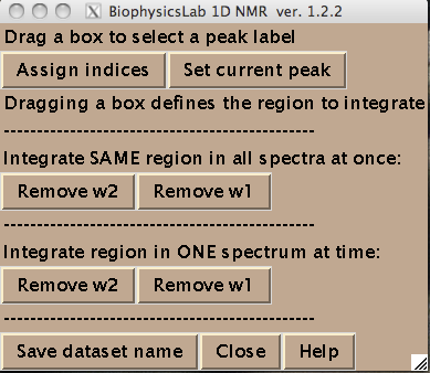
- All spectra in the titration series should have an integer index corresponding to the order in the titration series. Hit [Assign indices]. It brings up new window such as:
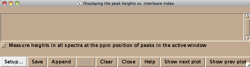
Technically this window belongs to a different Sparky extension (es in Evgenii menu). We invoke it to assign the indices to the 2D planes. Hit [Setup] to open the actual window where you spectra will be listed (both of these windows are based on standard Sparky Python extensions):
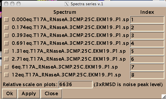
Add integers starting from 1 and click on check-boxes next to the spectra. These are the numbers your titration points will be known to MATLAB as. It is convenient if your file name begin with the number---then these fields are prefilled by Sparky from the first part of the file names.
(NOTE: Disregard 'Relative scale...' box. This number is not read by IDAP 1D NMR.)
IMPORTANT: All check boxes must be checked. Having any of them unchecked leads to the Python error. This is why you cannot have any other spectra in the project---only those you intend to extract data from !
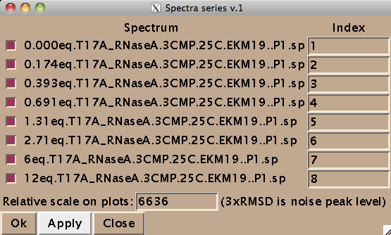
Now you should hit [Apply] and then [Close] to close this window. Hit [Close] in previous window as well and now you are left with just window from IDAP 1D NMR.
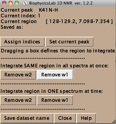
- You are ready to begin extraction of NMR line shapes. First you should select a peak the line shape 1D slices will belong to. Drag a rectangle around the peak and hit [Set current peak]. The captured peak name is shown in the window.
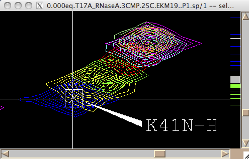
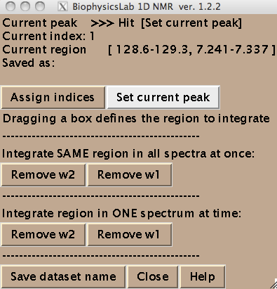
IDAP 1D NMR will use this name for all 1D slices from now on until you hit [Set current peak] again.
- Next step is to define a region to generate 1D slices. The main way is to look at an overlay of your spectra and drag a rectangle to encompass both free and bound peaks.
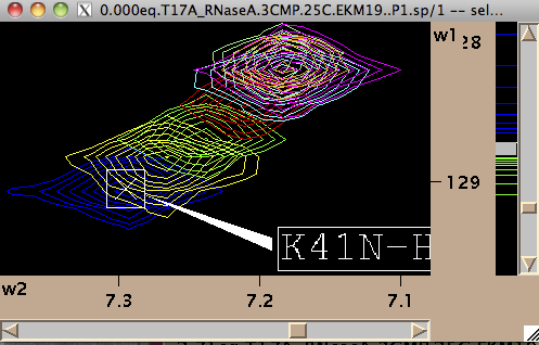
To integrate all of the at once hit [Remove w1] or [Remove w2] in 'Integrate SAME region in all spectra at once menu. Integration (removal) of w1 or w2 dimensions gives rise to two datasets for each peak: a 1D along w2 and w1, correspondingly.
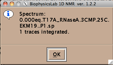
Once you hit Remove button the IDAP 1D NMR will automatically go through all spectra in the project, extract data, integrate along one dimension to leave w2 or w1, correspondingly, and save them individually for each . For example, once you hit Remove w2 button the IDAP 1D NMR makes a subfolder Data_for_IDAP/K41N-H_x_w1/. You will see a confirmation dialog for each spectrum it extracted data from:

The window tells you how many traces were taken from 2D plane and added together.
This is a quick way to extract line shapes from spectra with good S/N and little spectral crowding so it is possible to define a rectangular spectral region where only one peak of interest present throughout entire titration series.
- To obtain the best signal/noise ratio or avoid intrusion of nearby peaks into the integration, you may need to take only one 1D trace for each spectral slice. To do that you draw a very narrow rectangle going through the peak maxima along the desired dimension so your rectangle looks like a line. After that hit [Remove ...] button in Integrate region in ONE spectrum at a time part of menu. The confirmation window tells you whether you succeeded in taking just one trace. Now you want to go through spectra one by one and take 'custom' regions. (NOTE: to have this procedure work you should formally perform integration through Integrate SAME region in all spectra at once menu first---it creates the file structure on a disk).
An important feature is that you may re-take any slice at any time. You may begin analyzing your data in IDAP in MATLAB, then come back to Sparky and re-do extraction of the line shape for some selected spectrum. The data on a disk are updated for that specific slice while the rest of the data remains the same.
- IDAP 1D NMR output:
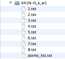
index.txt files contain raw integrated spectral data from each spectrum in a plain text format as an X-Y array. The index is the number you assigned to your spectra above. This data may be edited. If you prefer, you may produce this kind of data with any other program than Sparky and then read them by an object of IDAP_1D_NMR class.
- Hit [Set dataset name] to add the dataset name to the Data_for_IDAP/matlab.peaklist. This is a plain text file generated for your convenience so you could cut-and-paste dataset names from it into MATLAB notebooks.
Important considerations on preparation of line shape data and extraction strategies
- For successfull fitting of your data make sure to include the tails of the lorentzian line . If you don't include tails down to the baseline than you are not including full area of the line in calculations and it distorts the results.
- If you have any case of slow exchange (when peak is not moving) - use extraction procedure with the same region ( 'all spectra at once'). The reason is that if your line shape splits into two peaks - you must entirely encompass them with the rectangle, otherwise their relative intensities will be altered and that will certainly distort the fitting results. Therefore, use procedure of individual peak slicing ('Integrate region in ONE spectrum at a time') with caution or better not use it at all.
- In case of very large chemical shift changes in fast exchange - certainly use individual slicing option, because otherwise common rectangle will include too much of empty baseline and signal/noise ratio will be degraded (not mentioning increasing demand for RAM leading to 'Out of Memory' error in Matlab).