Tutorial 1. Simulation of 1D NMR line shape with IDAP

by Evgenii Kovrigin, 05/17/2011

Here I am showing coding steps to necessary to simulate 1D NMR line shapes for a simple R+L=RL process (U model). In this model we observe signals from R and RL while L is NMR-invisible (unlabeled with NMR-active isotopes). I will set some parameters for the U model and prepare a single 1D spectrum. I show how to export data and how to use both analytical and numeric solutions of the model.

I only intend to do simulation of a signal here. For fitting (later) we should use functionality of the TotalFit class

Clean up workspace
Set up model parameters for the 1D NMR line shape
Create NMR line shape dataset
Model, solver and solver options
Simulate ideal data
Simulate data with synthetic random noise
Save a dataset object
Example of using numeric solution of the models
Estimation of the NMR line parameters
Conclusions

Clean up workspace

(to avoid unwanted effects of old variable assignments)

close all
clear all

Set up model parameters for the 1D NMR line shape

I will be building a setup structure to be able to handle all these parameters as a single piece (therefore--exclusively for convenience)

setup.Rtotal    = 1e-3; % concentration of receptor, mol
setup.LRratio   = 0.75;    % ratio of the total concentration of ligand to receptor
setup.Log10_K_A        = log10(1e5); % equilibrium binding constant, 1/mol, in logarithmic form
setup.k_2_A    = 10;   % dissociation rate constant of the complex, 1/s
setup.w0_1      = 0;    % NMR frequency of the free receptor R, 1/s
setup.w0_2      = 200;  % NMR frequency of the bound complex RL, 1/s
setup.FWHH_1  = 20;     % line width at half height of the peak of R, 1/s
setup.FWHH_2  = 20;     % line width at half height of the peak of RL, 1/s
setup.ScaleFactor = 1;  % a multiplier for spectral amplitude (used only when fitting data)

Create NMR line shape dataset

Create data object for 1D NMR line shapes and list all models defined for this data type.

test1=NMRLineShapes1D('Simulation','Test_1');  % create a dataset object
test1.list_models()  % show existing models

ans =

Models defined in the object "Test_1" of type "1D NMR Line shapes"
-----------------------------------------------------------
Model 1:  "Lorentzian"
Model description
"Lorentzian function, analytical"
Model handle: line_shape_equations_1D.lorentzian
Current solver: analytical
Model parameters: 
1: Intensity     2: dw     3: w0     

Model 2:  "U-model"
Model description
"1D NMR line shape for the U model, no temperature/field dependence, analytical"
Model handle: line_shape_equations_1D.U_model_1D
Current solver: analytical
Model parameters: 
1: Rtotal     2: LRratio     3: log10(K_A)     4: k_2_A     5: w0_1     6: w0_2     7: FWHH_1     8: FWHH_2     9: ScaleFactor     

Model 3:  "U-model-LRcorrection"
Model description
"1D NMR line shape for the U model, no temperature/field dependence, with L/R correction, analytical"
Model handle: line_shape_equations_1D.U_model_1D_LRcorrection
Current solver: analytical
Model parameters: 
1: Rtotal     2: LRratio     3: log10(K_A)     4: k_2_A     5: w0_1     6: w0_2     7: FWHH_1     8: FWHH_2     9: ScaleFactor     10: LRcorrection     

Model 4:  "U-model-LRcorr-Jdoublet"
Model description
"1D NMR line shape for the U model split into a doublet with a constant J (1/s), no temperature/field dependence, with L/R correction, analytical"
Model handle: line_shape_equations_1D.U_model_1D_LRcorr_doublet
Current solver: analytical
Model parameters: 
1: Rtotal     2: LRratio     3: log10(K_A)     4: k_2_A     5: w0_1     6: w0_2     7: FWHH_1     8: FWHH_2     9: ScaleFactor     10: LRcorrection     11: Jconst     

Model 5:  "U_model_1D_LR_LB_SF"
Model description
"1D NMR line shape, U model, no T/B0 dep, with scaling factor, L/R correction and linear baseline, analytical"
Model handle: line_shape_equations_1D.U_model_1D_LR_LB_SF
Current solver: analytical
Model parameters: 
1: Rtotal     2: LRratio     3: log10(K_A)     4: k_2_A     5: w0_1     6: w0_2     7: FWHH_1     8: FWHH_2     9: ScaleFactor     10: LRcorrection     11: LB_a     12: LB_b     

Model 6:  "U_R-model"
Model description
"1D NMR line shape for the U-R model, no temperature/field dependence, analytical"
Model handle: line_shape_equations_1D.U_R_model_1D
Current solver: analytical
Model parameters: 
1: Rtotal     2: LRratio     3: log10(K_A)     4: log10(K_B)     5: k_2_A     6: k_2_B     7: w0_R     8: w0_Rstar     9: w0_RL     10: FWHH_R     11: FWHH_Rstar     12: FWHH_RL     13: ScaleFactor     

Model 7:  "U_R2-model"
Model description
"1D NMR line shape for the U-R2 model, no temperature/field dependence, fminbnd solver"
Model handle: line_shape_equations_1D.U_R2_model_1D
Current solver: analytical
Model parameters: 
1: Rtotal     2: LRratio     3: log10(K_A)     4: log10(K_B)     5: k_2_A     6: k_2_B     7: w0_R     8: w0_R2     9: w0_RL     10: FWHH_R     11: FWHH_R2     12: FWHH_RL     13: ScaleFactor     

Model 8:  "U_RL-model"
Model description
"1D NMR line shape for the U-RL model, no temperature/field dependence, analytical"
Model handle: line_shape_equations_1D.U_RL_model_1D
Current solver: analytical
Model parameters: 
1: Rtotal     2: LRratio     3: log10(K_A)     4: log10(K_B)     5: k_2_A     6: k_2_B     7: w0_R     8: w0_RL     9: w0_RLstar     10: FWHH_R     11: FWHH_RL     12: FWHH_RLstar     13: ScaleFactor     

Model 9:  "U_R2L2-model"
Model description
"1D NMR line shape for the U-R2L2 model, no temperature/field dependence, analytical"
Model handle: line_shape_equations_1D.U_R2L2_model_1D
Current solver: analytical
Model parameters: 
1: Rtotal     2: LRratio     3: log10(K_A)     4: log10(K_B)     5: k_2_A     6: k_2_B     7: w0_R     8: w0_RL     9: w0_R2L2     10: FWHH_R     11: FWHH_RL     12: FWHH_R2L2     13: ScaleFactor     

Model 10:  "U_R_L_RL-a-model"
Model description
"1D NMR line shape for the U-R-L-RL_a model, no temperature/field dependence, analytical"
Model handle: line_shape_equations_1D.U_R_L_RL_a_model_1D
Current solver: analytical
Model parameters: 
1: Rtotal     2: LRratio     3: log10(K_A1)     4: log10(K_B1)     5: log10(K_B2)     6: log10(K_B3)     7: k_2_A1     8: k_2_B1     9: k_2_B2     10: k_2_B3     11: w0_R     12: w0_Rstar     13: w0_RL     14: w0_RLstar     15: FWHH_R     16: FWHH_Rstar     17: FWHH_RL     18: FWHH_RLstar     19: ScaleFactor

Model, solver and solver options

First, we specify what model we want to use. For models that do not have analytical solutions we should specify a solver and its options. U model is soluble analytically so none of the options is required.

test1.set_active_model('U-model', 'analytical', 'no options')   % select a model, solver and its options
test1.show_active_model()

ans =

Active model:
Model 2:  "U-model"
Model description
"1D NMR line shape for the U model, no temperature/field dependence, analytical"
Model handle: line_shape_equations_1D.U_model_1D
Current solver: analytical
Model parameters: 
1: Rtotal     2: LRratio     3: log10(K_A)     4: k_2_A     5: w0_1     6: w0_2     7: FWHH_1     8: FWHH_2     9: ScaleFactor

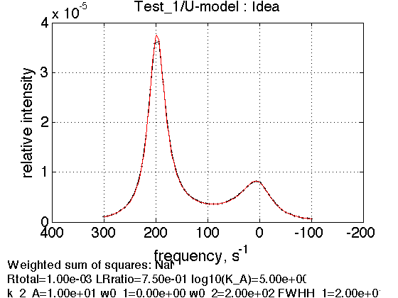
Simulate ideal data

Set range for X to extend beyond resonances

w_padding=100; % extend X axis by this amount beyond resonance positions
w_min= min([setup.w0_2,setup.w0_1])-w_padding;
w_max= max([setup.w0_2,setup.w0_1])+w_padding;
datapoints=50;  % Number of simulated 'experimental' data points
test1.set_X(linspace(w_min, w_max, datapoints));

Calculate ideal data: set noise RMSD to 0 for both X and Y in this example:

X_RMSD=0;
Y_RMSD=0;

Collect all parameters into a vector in the same order as model requires

parameters=[ setup.Rtotal  setup.LRratio   setup.Log10_K_A   setup.k_2_A  ...
              setup.w0_1   setup.w0_2   setup.FWHH_1  setup.FWHH_2  ...
              setup.ScaleFactor ];

Compute simulated line shape

tic;
test1.simulate_noisy_data(parameters, X_RMSD, Y_RMSD);
toc;
figure1=test1.plot_simulation('Ideal');

Elapsed time is 0.058935 seconds.

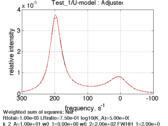
Adjust plotting ranges (if left empty - use automatic ranges in the plots)

test1.X_range=[min(test1.X) max(test1.X)];
test1.Y_range=[];
% re-plot
figure1=test1.plot_simulation('Adjusted');

Simulate data with synthetic random noise

Copy dataset

test2=test1.make_a_copy('Test_2');
% Now add noise
Signal_to_noise_ratio=20;
Y_RMSD=max(test2.Y)/Signal_to_noise_ratio;
test2.simulate_noisy_data(parameters, X_RMSD, Y_RMSD);
figure2=test2.plot_simulation('Noisy');

Save figure in all formats to a folder Tutorial_1/

results_output.output_figure(figure1,'Tutorial_1','U_model_ideal');
results_output.output_figure(figure2,'Tutorial_1','U_model_noisy');

Save a dataset object

We intend to do more work with this dataset later (try to fit it) therefore we need to save it to a disk. We will retrieve it in other tutorial using the following command temp=load('tutorial_1.mat'); test1=temp.test1; test2=temp.test2

save('tutorial_1.mat','test1', 'test2','setup');

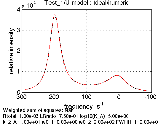
Example of using numeric solution of the models

As example of using models with numeric solution I am showing U model switched to the numeric operation

options=optimset('Diagnostics','off', ...
    'Display','off',...
    'LargeScale','on',...
    'LevenbergMarquardt', 'on',...
    'TolFun',1e-18,...
    'TolX',1e-18,...
    'MaxFunEvals', 1e9);
test1.set_active_model('U-model', 'lsqcurvefit', options)   % select a model, solver and its options
test1.show_active_model()

tic;
test1.simulate_noisy_data(parameters, 0, 0);
toc;
figure1=test1.plot_simulation('Ideal/numeric');

ans =

Active model:
Model 2:  "U-model"
Model description
"1D NMR line shape for the U model, no temperature/field dependence, analytical"
Model handle: line_shape_equations_1D.U_model_1D
Current solver: lsqcurvefit
Model parameters: 
1: Rtotal     2: LRratio     3: log10(K_A)     4: k_2_A     5: w0_1     6: w0_2     7: FWHH_1     8: FWHH_2     9: ScaleFactor     



Elapsed time is 0.372844 seconds.

Estimation of the NMR line parameters

NOTE: Fitting with real models should be done in TotalFit session!

Here I show how to estimate parameters of the line to generate starting parameters for fitting with complex models: line position, line width.

In this spectrum we got two lines. We need: (1) trim the datasets to leave only one line, and (2) fit with Lorentzian function to obtain estimates of line geometry.

% copy dataset first (to be able to freely mess it up!)
test3=test2.make_a_copy('parameter_estimation');
% trim data to retain only one line
X1=100;
X2=300;
test3.trim_data(X1,X2);
% show trimmed result
test3.X_range=[X1 X2];
test3.plot_data('Trimmed');

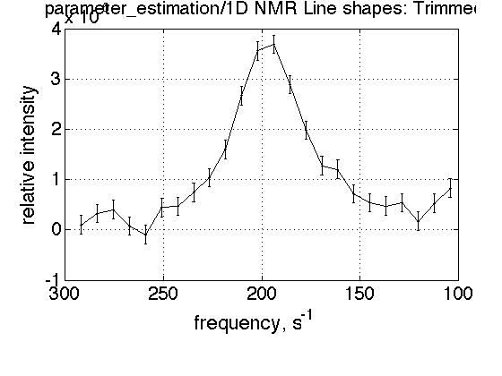
fit with lorentzian

mode='auto'; % use this if line is approximately centered in the window,
% otherwise use 'manual' and provide initial parameters I0, FWHH and w0
% (intensity, Full-width-at-half-height and frequency).
initial_parameters=[];
[ I0 FWHH w0 h1 h2] = test3.lorentzian_fit(mode, initial_parameters)
% save figures
results_output.output_figure(h1,'Tutorial_1','Lorentzian_initial_guess');
results_output.output_figure(h2,'Tutorial_1','Lorentzian_fit');

I0 =

   7.5855e-04


FWHH =

   40.2411


w0 =

  196.2076


h1 =

     6


h2 =

     7

This procedure is very handy when fitting real experimental data by providing automatic initial guess.

Conclusions

Here we explored basic manipulation of the line shape dataset.