Tutorial 6. Testing a new model

by Evgenii Kovrigin, 05/20/2011

IDAP is built to allow easy introduction of new mathematical models. Therefore, the models are numerous and have many versions for all imaginable purposes. A good practice in using new models is to assume that they contain both mathematical and programmatic glitches thus it is imperative to test their operation before using in data fitting. It is straightforward to test whether the model indeed works as expected by inspecting simulated signals.

The key concept is that, irrespective of the model inner workings, it describes a physical process that may be understood qualitatively without any calculations. What we need to do is to propose some set of conditions where we can qualitatively (or semi-quantitatively) predict the expected signal. If the model reasonably reproduces these test cases, chances are that it works well. Mathematical problems (incorrect assumptions, derivations, etc.) will manifest themselves in deviation of the modelled signal from expected features. Programmatic glitches result in a loss of common-sense behavior of the model when parameters are systematically changed.

NOTE: To ensure my own models are correctly derived I perform all derivations using MuPad (symbolic algebra package of MATLAB), which allows to document derivations very efficiently. The user is invited to examine and rerun these notebooks located in Mathematical_models/ folder.

This tutorial is an example of a common-sense-based testing of a standard model I am introducing in IDAP: U-R2, ligand binding coupled to dimerization of the receptor such that dimers do not bind the ligand. When I introduce other complex models I will place the testing documents in their respective folders in Mathematical_models/.

Model derivation
Test Computation of Equilibrium Concentrations
Test of NMR line shape calculations
Create NMR line shape dataset
Slow exchange in free receptor
Dilution of free receptor
Fast exchange in free receptor
A fully saturated receptor
Summary of individual plots
Create a titration series
Conclusions

Model derivation

We are not going through steps of model development here---only review them briefly and go to testing. The main steps in the model development are:

1. Develop mathematical equations to describe evolution of molecular species. The result is either analytical (closed-form) solution or an expression for solving numerically.

2. Create the model function in either code/+equilibrium_thermodynamic_equations or code/+differential_kinetic_equations packages.

3. Develop any additional math (such as kinetic matrices for NMR line shapes) to calculate expected experimental signal.

4. Create a model function that calculates signal using knowledge of molecular composition computed above. This is the function that will be called by a fitting routine to optimize parameters with respect to experimental data.

4. Add reference to this model in a data-specific subclass of the Dataset superclass.

After all this, we are ready to invoke the new model and see it in action.

close all
clear all

Here you will find all figures

figures_folder='U_R2_testing_figures';

Test Computation of Equilibrium Concentrations

Set some meaningful parameters

Rtotal=1e-3; % Receptor concentration, M
LRratio_array=[0 : 0.02 : 1.45]; % Array of L/R
K_a_A=1e6;  % Binding affinity constant
K_a_B=1e4;  % Dimerization constant

% Set appropriate options for the model (see model file for details)
model_numeric_solver='fminbnd'  ;

model_numeric_options=optimset('Diagnostics','off', ...
                    'Display','off',...
                    'TolX',1e-9,...
                    'MaxFunEvals', 1e9);

Important option here is TolX that sets termination tolerance on free ligand concentation in molar units. With our solution concentrations in 1e-3 range TolX should be set to some 1e-9.

Compute arrays for populations and plot

concentrations_array=[];
for counter=1:length(LRratio_array)
    % compute
    [concentrations species_names] = equilibrium_thermodynamic_equations.U_R2_model(...
        Rtotal, LRratio_array(counter), K_a_A, K_a_B,...
        model_numeric_solver, model_numeric_options);
    % collect
    concentrations_array = [concentrations_array ; concentrations];
end

Plot

Figure_title= 'U-R2 model';
X_range=[0 max(LRratio_array)+0.1 ]; % extend X just a bit past last point
Y_range=[ ]; % keep automatic scaling for Y
% display figure
figure_handle=equilibrium_thermodynamic_equations.plot_populations(...
    LRratio_array, concentrations_array, species_names, Figure_title, X_range, Y_range);
% save it
results_output.output_figure(figure_handle, figures_folder, 'Concentrations_plot');

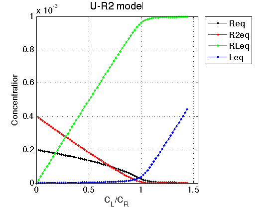
Observations The result is exactly what we expect from this model. In absence of a ligand the receptor exists in equilibrium between monomer, R, and a dimer, R2. Since one molecule of dimer is made of two monomers, the total concentration of a dimer has to be doubled to see concentration of the monomers in the dimer form. A sum of monomer concentration in free and dimer form is equal to Rtotal we set.

As ligand is added, the RL species is formed, leading to reduction of total concentration of the receptor. This reduction leads shifting of R<=>R2 equilibrium towards monomeric species such that above molar ratio L/R=0.8 the monomer becomes a major species in solution. This is the same effect as dilution of the receptor solution: progressive depletion of R2 population.

Once the receptor approaches saturation, the RL concentration approaches the Rtotal set above. At the same time, the free ligand begins to accumulate linearly with L/R molar ratio.

Conclusion

The model equilibrium_thermodynamic_equations.U_R2_model() works well.

Test of NMR line shape calculations

We will generate line shapes for in conditions where we can expect specific patterns. We will plot a spectrum at a specific solution conditions (we will not use Series of datasets for simplicity).

1. Ligand-free receptor in slow exchange should show two separate peaks with areas proportional to their equilibrium concentrations. This ratio should change upon dilution in favor of the monomer. NOTE: NMR intensity is proportional to concentrations of NMR-active spins so it will track concentration of monomers in monomeric and dimeric structures.

2. Fast exchange in the same setting should reveal population-weighted average peak. Here, again, the concentration of monomers in free and dimeric form will be important---not the concentration of dimeric species. Similarly, dilution would lead to a shift of a peak towards frequency of monomeric species.

3. Addition of saturating concentration of ligand should give us a single peak at the RL frequency.

Create NMR line shape dataset

Create data object for 1D NMR line shapes

test1=NMRLineShapes1D('Simulation','Test_1');
test1.set_active_model('U_R2-model', model_numeric_solver, model_numeric_options)
test1.show_active_model() % to look up necessary parameters of the model

ans =

Active model:
Model 7:  "U_R2-model"
Model description
"1D NMR line shape for the U-R2 model, no temperature/field dependence, fminbnd solver"
Model handle: line_shape_equations_1D.U_R2_model_1D
Current solver: fminbnd
Model parameters: 
1: Rtotal     2: LRratio     3: log10(K_A)     4: log10(K_B)     5: k_2_A     6: k_2_B     7: w0_R     8: w0_R2     9: w0_RL     10: FWHH_R     11: FWHH_R2     12: FWHH_RL     13: ScaleFactor

Set range for X to extend beyond resonances

w_min= -300;
w_max= 500;
datapoints=100;  % Does not matter much because smooth curve is anyway calculated
test1.set_X(linspace(w_min, w_max, datapoints));

Set fixed plotting ranges for easier comparison If we do not set ranges they will be chosen automatically for each graph

test1.X_range=[w_min w_max]; % this sets display range in the plots
test1.Y_range=[0 8e-5]; % this sets display range in the plots

Calculate ideal data: set noise RMSD to 0 for both X and Y

X_RMSD=0;
Y_RMSD=0;

Slow exchange in free receptor

Use the same thermodynamic parameters as above. Add spectral and kinetic parameters:

LRratio = 0.01 ;  % NOTE: for a numeric model this value has to be >=0.01
Log10_K_A = log10(K_a_A);
Log10_K_B = log10(K_a_B);
k_2_A    = 1;   % dissociation rate constant of the complex, 1/s
k_2_B    = 1;   % dissociation rate constant of the receptor dimer, 1/s
w0_R     = -200;    % NMR frequency of the free receptor R, 1/s
w0_R2    = 200;  % NMR frequency of the dimer R2, 1/s
w0_RL    = 400;  % NMR frequency of the bound complex RL, 1/s
FWHH_R   = 20;     % line width at half height of the peak of R, 1/s
FWHH_R2  = 20;     % line width at half height of the peak of R2, 1/s
FWHH_RL  = 20;     % line width at half height of the peak of RL, 1/s
ScaleFactor = 1;  % a multiplier for spectral amplitude (used only when fitting data)

% compute equilbrium concentrations
[concentrations species_names] = equilibrium_thermodynamic_equations.U_R2_model(...
        Rtotal, LRratio, K_a_A, K_a_B,...
        model_numeric_solver, model_numeric_options)


% plot line shapes
parameters=[ Rtotal  LRratio   Log10_K_A   Log10_K_B  k_2_A  k_2_B ...
     w0_R  w0_R2  w0_RL  FWHH_R  FWHH_R2  FWHH_RL  ScaleFactor ];


test1.simulate_noisy_data(parameters, X_RMSD, Y_RMSD);
figure_handle=test1.plot_simulation('Slow: free R');
results_output.output_figure(figure_handle, figures_folder, 'Slow_concentrated_R');

concentrations =

   1.0e-03 *

    0.1993    0.3973    0.0100    0.0000


species_names = 

    'Req'    'R2eq'    'RLeq'    'Leq'

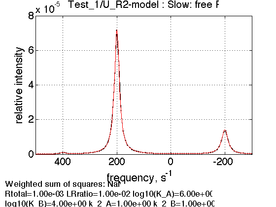
Expected ratio of R2 peak to R peak is 4:1 corresponding to number of spins experiencing dimeric and monomeric environment.

Prepare TotalFit session for easy display of many graphs

storage_session=TotalFit('All_tests');
% set aside for plotting later
storage_session.copy_dataset_into_array(test1);

Dilution of free receptor

Rtotal=1e-4;

% compute equilbrium concentrations
[concentrations species_names] = equilibrium_thermodynamic_equations.U_R2_model(...
        Rtotal, LRratio, K_a_A, K_a_B,...
        model_numeric_solver, model_numeric_options)



parameters=[ Rtotal  LRratio   Log10_K_A   Log10_K_B  k_2_A  k_2_B ...
     w0_R  w0_R2  w0_RL  FWHH_R  FWHH_R2  FWHH_RL  ScaleFactor ];


test1.simulate_noisy_data(parameters, X_RMSD, Y_RMSD);
figure_handle=test1.plot_simulation('Slow: 1/10 R');
results_output.output_figure(figure_handle, figures_folder, 'Slow_diluted_R');
% set aside for plotting later
storage_session.copy_dataset_into_array(test1);

concentrations =

   1.0e-04 *

    0.4965    0.2466    0.0098    0.0002


species_names = 

    'Req'    'R2eq'    'RLeq'    'Leq'

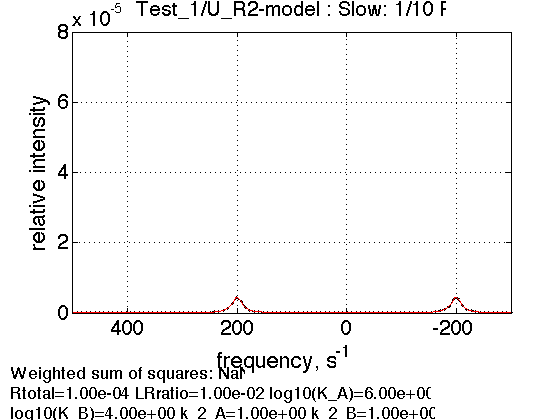
When receptor is diluted we see relative reduction in population of R2 with respect to R: peak areas are almost equal now reflecting similar number of spins in each environment (total concentration of spins, obviously, dropped due to dilution).

Fast exchange in free receptor

Diluted

k_2_B=1000;
parameters=[ Rtotal  LRratio   Log10_K_A   Log10_K_B  k_2_A  k_2_B ...
     w0_R  w0_R2  w0_RL  FWHH_R  FWHH_R2  FWHH_RL  ScaleFactor ];


test1.simulate_noisy_data(parameters, X_RMSD, Y_RMSD);
figure_handle=test1.plot_simulation('Fast: 1/10 R');
results_output.output_figure(figure_handle, figures_folder, 'Fast_diluted_R');
% set aside for plotting later
storage_session.copy_dataset_into_array(test1);

The weighted average peak is almost in the middle with a very slight shift towards the monomer, because it has very slightly more spins than dimer in these conditions

Concentrated: Return to the original condition

Rtotal=1e-3;

% compute equilbrium concentrations
[concentrations species_names] = equilibrium_thermodynamic_equations.U_R2_model(...
        Rtotal, LRratio, K_a_A, K_a_B,...
        model_numeric_solver, model_numeric_options)



parameters=[ Rtotal  LRratio   Log10_K_A   Log10_K_B  k_2_A  k_2_B ...
     w0_R  w0_R2  w0_RL  FWHH_R  FWHH_R2  FWHH_RL  ScaleFactor ];


test1.simulate_noisy_data(parameters, X_RMSD, Y_RMSD);
figure_handle=test1.plot_simulation('Fast: 1/1 R');
results_output.output_figure(figure_handle, figures_folder, 'Fast_concentrated_R');
% set aside for plotting later
storage_session.copy_dataset_into_array(test1);

concentrations =

   1.0e-03 *

    0.1993    0.3973    0.0100    0.0000


species_names = 

    'Req'    'R2eq'    'RLeq'    'Leq'

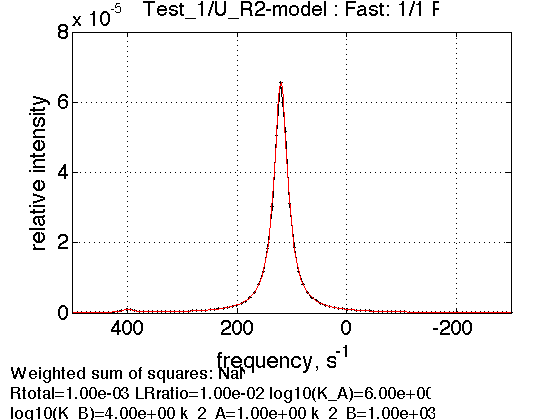
The peak is roughly at 4:1 weighted position in favor of a dimer

A fully saturated receptor

LRratio = 10 ;
parameters=[ Rtotal  LRratio   Log10_K_A   Log10_K_B  k_2_A  k_2_B ...
     w0_R  w0_R2  w0_RL  FWHH_R  FWHH_R2  FWHH_RL  ScaleFactor ];

test1.simulate_noisy_data(parameters, X_RMSD, Y_RMSD);
figure_handle=test1.plot_simulation('saturated RL');
results_output.output_figure(figure_handle, figures_folder, 'Saturated_RL');
% set aside for plotting later
storage_session.copy_dataset_into_array(test1);

We observe a peak at a frequency of bound form

Summary of individual plots

storage_session.define_series('All-tests',1:length(storage_session.dataset_array));
figure_handle=storage_session.plot_1D_series('All-tests', 'All tests', 0);
results_output.output_figure(figure_handle, figures_folder, 'All_tests');

This is a comparison graph of all previous plots

Create a titration series

(see Tutorial 3 for details) Choose parameters

ZERO_LRratio= 0.01; % This number cannot be too small---the model is numeric and will NOT converge!
LRratio_vector=[ZERO_LRratio  0.2   0.4   0.6  0.8   1.0   1.2   1.4 ];


% choose the same parameters as above
session_name='Series';
session=TotalFit(session_name);
series_name='U-R2_simulation';
dataset_class_name='NMRLineShapes1D';
model_name='U_R2-model';
number_of_datasets=length(LRratio_vector);
X_column=test1.X; % use the same range

% create TotalFit session
session.create_simulation_series(series_name, dataset_class_name, model_name, ...
                 model_numeric_solver, model_numeric_options,...
                 number_of_datasets, X_column);

session.initialize_relation_matrix(sprintf('%s.all_datasets.txt', session_name));

% link parameters
parameter_number_array=[ 1    3 4 5 6 7 8 9 10 11 12 13];
session.batch_link_parameters_in_series(series_name, parameter_number_array);
session.generate_fitting_environment(sprintf('%s.fitting_environment.txt', session_name))

% prepare parameters
first_dataset_index=session.dataset_index(series_name,1);
FAKE_VALUE=1E-6;  % individual (unlinked) parameters: to be assigned later

ideal_parameters=[ Rtotal  FAKE_VALUE   Log10_K_A   Log10_K_B  k_2_A  k_2_B ...
     w0_R  w0_R2  w0_RL  FWHH_R  FWHH_R2  FWHH_RL  ScaleFactor ];

% prepare formal limits
fake_limits=zeros(1,length(ideal_parameters));
Monte_Carlo_range_min=fake_limits;
Monte_Carlo_range_max=fake_limits;
parameter_limits_min=fake_limits;
parameter_limits_max=fake_limits;

% assign
session.assign_parameter_values(first_dataset_index, ideal_parameters, ...
        Monte_Carlo_range_min, Monte_Carlo_range_max, parameter_limits_min, parameter_limits_max);

% Assign unlinked LRratio and ranges
parameter_number=2;
values_array=LRratio_vector;

unlinked_fake_ranges=zeros(1,number_of_datasets);
MonteCarlo_range_min_array=unlinked_fake_ranges;
MonteCarlo_range_max_array=unlinked_fake_ranges;
parameter_limits_min_array=unlinked_fake_ranges;
parameter_limits_max_array=unlinked_fake_ranges;

session.assign_unlinked_parameter_in_series(...
             series_name, parameter_number, values_array, ...
             MonteCarlo_range_min_array, MonteCarlo_range_max_array, ...
             parameter_limits_min_array, parameter_limits_max_array);

% Simulate series
X_standard_dev=0;
Y_standard_dev=1e-8;  % something really small
session.simulate_series(series_name, X_standard_dev, Y_standard_dev);

% Plot
Y_offset_percent=10;  % to offset figures vertically for easier viewing
% set plotting ranges
X_range=test1.X_range;  % use old
Y_range=[];  % automatic
session.set_XY_ranges_series(series_name, X_range, Y_range)
figure_handle=session.plot_1D_series(series_name, session.name, Y_offset_percent);
results_output.output_figure(figure_handle, figures_folder, 'Series');

Dataset listing is written to "Series.all_datasets.txt".

Fitting environment saved in Series.fitting_environment.txt.

ans =

New parameter relations (indexed as in all_parameters vector):

[1]     1:Rtotal | 2:Rtotal | 3:Rtotal | 4:Rtotal | 5:Rtotal | 6:Rtotal | 7:Rtotal | 8:Rtotal
[2]     1:LRratio
[3]     1:log10(K_A) | 2:log10(K_A) | 3:log10(K_A) | 4:log10(K_A) | 5:log10(K_A) | 6:log10(K_A) | 7:log10(K_A) | 8:log10(K_A)
[4]     1:log10(K_B) | 2:log10(K_B) | 3:log10(K_B) | 4:log10(K_B) | 5:log10(K_B) | 6:log10(K_B) | 7:log10(K_B) | 8:log10(K_B)
[5]     1:k_2_A | 2:k_2_A | 3:k_2_A | 4:k_2_A | 5:k_2_A | 6:k_2_A | 7:k_2_A | 8:k_2_A
[6]     1:k_2_B | 2:k_2_B | 3:k_2_B | 4:k_2_B | 5:k_2_B | 6:k_2_B | 7:k_2_B | 8:k_2_B
[7]     1:w0_R | 2:w0_R | 3:w0_R | 4:w0_R | 5:w0_R | 6:w0_R | 7:w0_R | 8:w0_R
[8]     1:w0_R2 | 2:w0_R2 | 3:w0_R2 | 4:w0_R2 | 5:w0_R2 | 6:w0_R2 | 7:w0_R2 | 8:w0_R2
[9]     1:w0_RL | 2:w0_RL | 3:w0_RL | 4:w0_RL | 5:w0_RL | 6:w0_RL | 7:w0_RL | 8:w0_RL
[10]     1:FWHH_R | 2:FWHH_R | 3:FWHH_R | 4:FWHH_R | 5:FWHH_R | 6:FWHH_R | 7:FWHH_R | 8:FWHH_R
[11]     1:FWHH_R2 | 2:FWHH_R2 | 3:FWHH_R2 | 4:FWHH_R2 | 5:FWHH_R2 | 6:FWHH_R2 | 7:FWHH_R2 | 8:FWHH_R2
[12]     1:FWHH_RL | 2:FWHH_RL | 3:FWHH_RL | 4:FWHH_RL | 5:FWHH_RL | 6:FWHH_RL | 7:FWHH_RL | 8:FWHH_RL
[13]     1:ScaleFactor | 2:ScaleFactor | 3:ScaleFactor | 4:ScaleFactor | 5:ScaleFactor | 6:ScaleFactor | 7:ScaleFactor | 8:ScaleFactor
[14]   n/a
[15]     2:LRratio
[16]   n/a
[17]   n/a
[18]   n/a
[19]   n/a
[20]   n/a
[21]   n/a
[22]   n/a
[23]   n/a
[24]   n/a
[25]   n/a
[26]   n/a
[27]   n/a
[28]     3:LRratio
[29]   n/a
[30]   n/a
[31]   n/a
[32]   n/a
[33]   n/a
[34]   n/a
[35]   n/a
[36]   n/a
[37]   n/a
[38]   n/a
[39]   n/a
[40]   n/a
[41]     4:LRratio
[42]   n/a
[43]   n/a
[44]   n/a
[45]   n/a
[46]   n/a
[47]   n/a
[48]   n/a
[49]   n/a
[50]   n/a
[51]   n/a
[52]   n/a
[53]   n/a
[54]     5:LRratio
[55]   n/a
[56]   n/a
[57]   n/a
[58]   n/a
[59]   n/a
[60]   n/a
[61]   n/a
[62]   n/a
[63]   n/a
[64]   n/a
[65]   n/a
[66]   n/a
[67]     6:LRratio
[68]   n/a
[69]   n/a
[70]   n/a
[71]   n/a
[72]   n/a
[73]   n/a
[74]   n/a
[75]   n/a
[76]   n/a
[77]   n/a
[78]   n/a
[79]   n/a
[80]     7:LRratio
[81]   n/a
[82]   n/a
[83]   n/a
[84]   n/a
[85]   n/a
[86]   n/a
[87]   n/a
[88]   n/a
[89]   n/a
[90]   n/a
[91]   n/a
[92]   n/a
[93]     8:LRratio
[94]   n/a
[95]   n/a
[96]   n/a
[97]   n/a
[98]   n/a
[99]   n/a
[100]   n/a
[101]   n/a
[102]   n/a
[103]   n/a
[104]   n/a

Summary of datasets with lookup vectors (position of each parameter in all_parameter vector)
--------
Dataset 1/U-R2_simulation-1,  model "U_R2-model"
Parameters          :    Rtotal    LRratio    log10(K_A)    log10(K_B)    k_2_A    k_2_B    w0_R    w0_R2    w0_RL    FWHH_R    FWHH_R2    FWHH_RL    ScaleFactor
Lookup vector       :   1   2   3   4   5   6   7   8   9   10   11   12   13

Dataset 2/U-R2_simulation-2,  model "U_R2-model"
Parameters          :    Rtotal    LRratio    log10(K_A)    log10(K_B)    k_2_A    k_2_B    w0_R    w0_R2    w0_RL    FWHH_R    FWHH_R2    FWHH_RL    ScaleFactor
Lookup vector       :   1   15   3   4   5   6   7   8   9   10   11   12   13

Dataset 3/U-R2_simulation-3,  model "U_R2-model"
Parameters          :    Rtotal    LRratio    log10(K_A)    log10(K_B)    k_2_A    k_2_B    w0_R    w0_R2    w0_RL    FWHH_R    FWHH_R2    FWHH_RL    ScaleFactor
Lookup vector       :   1   28   3   4   5   6   7   8   9   10   11   12   13

Dataset 4/U-R2_simulation-4,  model "U_R2-model"
Parameters          :    Rtotal    LRratio    log10(K_A)    log10(K_B)    k_2_A    k_2_B    w0_R    w0_R2    w0_RL    FWHH_R    FWHH_R2    FWHH_RL    ScaleFactor
Lookup vector       :   1   41   3   4   5   6   7   8   9   10   11   12   13

Dataset 5/U-R2_simulation-5,  model "U_R2-model"
Parameters          :    Rtotal    LRratio    log10(K_A)    log10(K_B)    k_2_A    k_2_B    w0_R    w0_R2    w0_RL    FWHH_R    FWHH_R2    FWHH_RL    ScaleFactor
Lookup vector       :   1   54   3   4   5   6   7   8   9   10   11   12   13

Dataset 6/U-R2_simulation-6,  model "U_R2-model"
Parameters          :    Rtotal    LRratio    log10(K_A)    log10(K_B)    k_2_A    k_2_B    w0_R    w0_R2    w0_RL    FWHH_R    FWHH_R2    FWHH_RL    ScaleFactor
Lookup vector       :   1   67   3   4   5   6   7   8   9   10   11   12   13

Dataset 7/U-R2_simulation-7,  model "U_R2-model"
Parameters          :    Rtotal    LRratio    log10(K_A)    log10(K_B)    k_2_A    k_2_B    w0_R    w0_R2    w0_RL    FWHH_R    FWHH_R2    FWHH_RL    ScaleFactor
Lookup vector       :   1   80   3   4   5   6   7   8   9   10   11   12   13

Dataset 8/U-R2_simulation-8,  model "U_R2-model"
Parameters          :    Rtotal    LRratio    log10(K_A)    log10(K_B)    k_2_A    k_2_B    w0_R    w0_R2    w0_RL    FWHH_R    FWHH_R2    FWHH_RL    ScaleFactor
Lookup vector       :   1   93   3   4   5   6   7   8   9   10   11   12   13

This is an expected result. Binding in slow exchange leads to appearance of RL resonance, which gradually increases in intensity. Fast exchange between monomer and a dimer leads to a single population-weighted average peak that shifts towards monomer resonance frequency upon titration (as concentration of unliganded R decreases).

Conclusions

The U-R2 model for NMR 1D line shapes works as expected.