![]()
![]()
B family models (derivation)
Binding of two ligand molecules to one receptor monomer including bidentate
ligand binding; macroscopic and microscopic consideration.
Evgenii L. Kovrigin
12-10-2014
Updates:
1/13/2015 - rename transitions to have internal isomerization ("hopping") transition called "B" in all models and bi-dentate binding transition called "C"
2. Basic equilibrium equations
3. Analysis of statistical effects on binding and kinetic constants
4. Derivation of equations for concentrations of species
5. Prepare equations for a numeric solution
6. Save results on disk for future use
1. define thermodynamic and kinetic equations for binding of two ligands to one receptor molecule model.
2. analyze relationship between microscopic and macroscopic constants.
3. prepare equations for calculations of equilibrium concentrations in the titration experiment.
Derivation of kinetic matrices for microscopic models is done separately in Mathematical_models/NMR_line_shape_models/1D
Analysis of the solutions will be done separately.
clean up workspace
reset()
Set path to save results into:
NOTE: make sure the path ends with slash character "/".
ProjectName:="B_family_models_derivation";
CurrentPath:="/Volumes/Leopard_Partition/Users/kovrigin/Documents/Workspace/Global Analysis/IDAP/Mathematical_models/Equilibrium_thermodynamic_models/B_family_models/";
![]()
![]()
We will be considering the system two ways: using macroscopic and microscopic binding constants [1]. Overall, these are two completely equivalent treatments but interpretation in terms of mechanistic events is only available for microscopic constants.
1. Cantor, C.R. and Schimmel, P.R., Biophysical Chemistry. Part III. The behavior of biological macromolecules. Vol. III. 1980, New York: W.H. Freeman and Co. 360.
From: Equilibrium_thermodynamic_models/B_family_models/B
The more complicated version where the ligand is bidentate and capable of binding at both sites:
From Equilibrium_thermodynamic_models/B_family_models/B-bidentateL
This may be viewed as a combination of B and U-RL model (not exactly, though, because there are three isomerization transitions in B-bidentateL-micro.
1/13/2015:
Name replacement schedule:
B_1_I_I -> C_I_I
B_1_I -> C_I
B_1 -> B
B_2 -> B
Binding and isomerization constants
NOTE 1: All binding constants I am using are association constants.
NOTE 2: These relationships serve as restraints for solve(), but not restrict these values in calculations!
Macroscopic equilibrium constants
K_A_1
K_A_1 ;
assumeAlso(K_A_1 > 0):
assumeAlso(K_A_1 , R_):
![]()
K_A_2
K_A_2 ;
assumeAlso(K_A_2 > 0):
assumeAlso(K_A_2 , R_):
![]()
Macroscopic kinetic constants
k_1_A_1
k_1_A_1 ;
assumeAlso(k_1_A_1 > 0):
assumeAlso(k_1_A_1 , R_):
![]()
k_2_A_1
k_2_A_1 ;
assumeAlso(k_2_A_1 > 0):
assumeAlso(k_2_A_1 , R_):
![]()
k_1_A_2
k_1_A_2 ;
assumeAlso(k_1_A_2 > 0):
assumeAlso(k_1_A_2 , R_):
![]()
k_2_A_2
k_2_A_2 ;
assumeAlso(k_2_A_2 > 0):
assumeAlso(k_2_A_2 , R_):
![]()
Microscopic equilibrium binding constants
K_A_1_I
K_A_1_I ;
assumeAlso(K_A_1_I > 0):
assumeAlso(K_A_1_I , R_):
![]()
K_A_1_I_I
K_A_1_I_I ;
assumeAlso(K_A_1_I_I > 0):
assumeAlso(K_A_1_I_I , R_):
![]()
K_A_2_I
K_A_2_I ;
assumeAlso(K_A_2_I > 0):
assumeAlso(K_A_2_I , R_):
![]()
K_A_2_I_I
K_A_2_I_I ;
assumeAlso(K_A_2_I_I > 0):
assumeAlso(K_A_2_I_I , R_):
![]()
Microscopic equilibrium isomerization constants
K_C_I
K_C_I ;
assumeAlso(K_C_I > 0):
assumeAlso(K_C_I , R_):
![]()
K_C_I_I
K_C_I_I ;
assumeAlso(K_C_I_I > 0):
assumeAlso(K_C_I_I , R_):
![]()
K_B
K_B ;
assumeAlso(K_B > 0):
assumeAlso(K_B , R_):
![]()
Microscopic binding/dissociation rate constants
k_1_A_1_I
k_1_A_1_I ;
assumeAlso(k_1_A_1_I > 0):
assumeAlso(k_1_A_1_I , R_):
![]()
k_2_A_1_I
k_2_A_1_I ;
assumeAlso(k_2_A_1_I > 0):
assumeAlso(k_2_A_1_I , R_):
![]()
k_1_A_1_I_I
k_1_A_1_I_I ;
assumeAlso(k_1_A_1_I_I > 0):
assumeAlso(k_1_A_1_I_I , R_):
![]()
k_2_A_1_I_I
k_2_A_1_I_I ;
assumeAlso(k_2_A_1_I_I > 0):
assumeAlso(k_2_A_1_I_I , R_):
![]()
k_1_A_2_I_I
k_1_A_2_I_I ;
assumeAlso(k_1_A_2_I_I > 0):
assumeAlso(k_1_A_2_I_I , R_):
![]()
k_2_A_2_I_I
k_2_A_2_I_I ;
assumeAlso(k_2_A_2_I_I > 0):
assumeAlso(k_2_A_2_I_I , R_):
![]()
k_1_A_2_I
k_1_A_2_I ;
assumeAlso(k_1_A_2_I > 0):
assumeAlso(k_1_A_2_I , R_):
![]()
k_2_A_2_I
k_2_A_2_I ;
assumeAlso(k_2_A_2_I > 0):
assumeAlso(k_2_A_2_I , R_):
![]()
Microscopic isomerization rate constants
k_1_C_I_I
k_1_C_I_I ;
assumeAlso(k_1_C_I_I > 0):
assumeAlso(k_1_C_I_I , R_):
![]()
k_2_C_I_I
k_2_C_I_I ;
assumeAlso(k_2_C_I_I > 0):
assumeAlso(k_2_C_I_I , R_):
![]()
k_1_C_I
k_1_C_I ;
assumeAlso(k_1_C_I > 0):
assumeAlso(k_1_C_I , R_):
![]()
k_2_C_I
k_2_C_I ;
assumeAlso(k_2_C_I > 0):
assumeAlso(k_2_C_I , R_):
![]()
k_1_B
k_1_B ;
assumeAlso(k_1_B > 0):
assumeAlso(k_1_B , R_):
![]()
k_2_B
k_2_B ;
assumeAlso(k_2_B > 0):
assumeAlso(k_2_B , R_):
![]()
Total concentrations
Rtot - total concentration of the receptor
Rtot;
assumeAlso(Rtot>0):
assumeAlso(Rtot,R_):
![]()
Ltot - total concentration of a ligand
Ltot;
assumeAlso(Ltot>0):
assumeAlso(Ltot,R_):
![]()
Equilibrium concentrations
Req - free receptor
Req;
assumeAlso(Req>0):
assumeAlso(Req<Rtot):
assumeAlso(Req,R_):
![]()
Leq - free ligand
Leq;
assumeAlso(Leq>0):
assumeAlso(Leq<Ltot):
assumeAlso(Leq,R_):
![]()
RLeq - equlibrium conentration of single-bound species in the mAcroscopic view
(all of them summed together; they are indistinguishable in this view)
RLeq;
assumeAlso(RLeq>0):
assumeAlso(RLeq<Rtot):
assumeAlso(RLeq<Ltot):
assumeAlso(RLeq,R_):
![]()
RL_2eq - double bound species
RL_2eq;
assumeAlso(RL_2eq>0):
assumeAlso(RL_2eq<Rtot):
assumeAlso(RL_2eq<Ltot/2):
assumeAlso(RL_2eq,R_):
![]()
Microscopic equilibrium concentrations
(in this view we can independently measure their concentrations)
RL_Ieq
RL_Ieq;
assumeAlso(RL_Ieq>0):
assumeAlso(RL_Ieq<Rtot):
assumeAlso(RL_Ieq<Ltot):
assumeAlso(RL_Ieq,R_):
![]()
RL_I_Ieq
RL_I_Ieq;
assumeAlso(RL_I_Ieq>0):
assumeAlso(RL_I_Ieq<Rtot):
assumeAlso(RL_I_Ieq<Ltot):
assumeAlso(RL_I_Ieq,R_):
![]()
RL_b_ieq
RL_b_ieq;
assumeAlso(RL_b_ieq>0):
assumeAlso(RL_b_ieq<Rtot):
assumeAlso(RL_b_ieq<Ltot):
assumeAlso(RL_b_ieq,R_):
![]()
Check if all names are correctly entered:
anames(Properties,User);

2. Basic equilibrium equations
Goal: I will try to express analytical [L] from equation for a total concentration of a receptor or use the expression for a numeric solution if analytical is not possible
2.1 Equations for the mAcroscopic B model
Total concentration (mass balance) equations:
eq2_1_1_BmAcro:= Rtot = Req + RLeq + RL_2eq;
eq2_1_2_BmAcro:= Ltot = Leq + RLeq + 2* RL_2eq
![]()
![]()
Equilibrium thermodynamics equations for independent constants
eq2_1_3_BmAcro:= K_A_1 = RLeq / (Req*Leq);
![]()
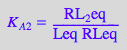
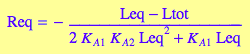
eq2_1_4_BmAcro:= K_A_2 = RL_2eq / (RLeq*Leq);

2.2 Equations for the microscopic B model (mono-dentate binding only)
Total concentration (mass balance) equations:
eq2_2_1_Bmicro:= RLeq = RL_Ieq + RL_I_Ieq;
![]()
eq2_2_2_Bmicro:= Rtot = Req + RLeq + RL_2eq;
![]()
eq2_2_3_Bmicro:= Ltot = Leq + RLeq + 2* RL_2eq;
![]()
Equilibrium thermodynamics equations for independent constants:
eq2_2_4_Bmicro:= K_A_1_I = RL_Ieq / (Req*Leq);

eq2_2_5_Bmicro:= K_A_1_I_I = RL_I_Ieq / (Req*Leq);

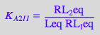
eq2_2_6_Bmicro:= K_A_2_I_I = RL_2eq / (RL_Ieq*Leq);

Dependent constants: K_A_2_I and K_B (from thermodynamic cycles)
eq2_2_7_Bmicro:= K_A_2_I = K_A_1_I * K_A_2_I_I / K_A_1_I_I
![]()
eq2_2_8_Bmicro:= K_B = K_A_1_I_I / K_A_1_I
![]()
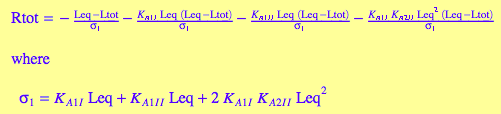
2.3 Equations for the microscopic B-bidentateL model (bi-dentate ligand)
Total concentration (mass balance) equations:
eq2_3_1_Bbidentate:= RLeq = RL_Ieq + RL_I_Ieq + RL_b_ieq;
![]()
eq2_3_2_Bbidentate:= Rtot = Req + RLeq + RL_2eq;
![]()
eq2_3_3_Bbidentate:= Ltot = Leq + RLeq + 2*RL_2eq;
![]()
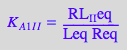
Equilibrium thermodynamics equations for independent constants:
eq2_3_4_Bbidentate:= K_A_1_I = RL_Ieq / (Req*Leq);
eq2_3_5_Bbidentate:= K_A_1_I_I = RL_I_Ieq / (Req*Leq);

eq2_3_6_Bbidentate:= K_A_2_I_I = RL_2eq / (RL_Ieq*Leq);

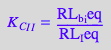
eq2_3_7_Bbidentate:= K_C_I_I = RL_b_ieq / (RL_Ieq);

Dependent: K_A_2_I, K_C_I, and K_B (from thermodynamic cycles)
eq2_3_8_Bbidentate:= K_A_2_I = K_A_1_I * K_A_2_I_I / K_A_1_I_I
![]()
eq2_3_9_Bbidentate:= K_C_I = K_A_1_I * K_C_I_I / K_A_1_I_I
![]()
eq2_3_10_Bbidentate:= K_B = K_A_1_I_I / K_A_1_I
![]()
3. Analysis of statistical effects on binding and kinetic constants
"Statistical effects" implies differences between macroscopic and microscopic constants due to the fact that in the macroscopic view we cannot discriminate individual single-bound species [1]. Standard approach: express equilbrium concentrations of those species you will not discriminate in the macroscopic treatment ("microscopic species") and then substitute into the mass balance equation for the single-bound species. Then substitute the result into the macroscopic association constant expression.
[1]. Cantor, C.R. and Schimmel, P.R., Biophysical Chemistry. Part III. The behavior of biological macromolecules. Vol. III. 1980, New York: W.H. Freeman and Co. 360.
3.1 Microscopic B model (mono-dentate ligand binding)
Mass balance
eq2_2_1_Bmicro
![]()
Macroscopic steps
eq2_1_3_BmAcro
![]()
eq2_1_4_BmAcro

First ligand-binding step:
eq2_2_4_Bmicro:
solve(%, RL_Ieq):
%[1][1]:
eq3_1_1_Bmicro:= RL_Ieq = %
![]()
eq2_2_5_Bmicro:
solve(%, RL_I_Ieq):
%[1][1]:
eq3_1_2_Bmicro:= RL_I_Ieq = %
![]()
Substitue into the mass balance for single-bound species
eq2_2_1_Bmicro:
% | eq3_1_1_Bmicro | eq3_1_2_Bmicro:
eq3_1_3_Bmicro:= %
![]()
Substitute into the expression for the mAcroscopic association constant
eq2_1_3_BmAcro:
% | eq3_1_3_Bmicro:
normal(%):
eq3_1_4_Bmicro:= %
![]()
=> this is a relationship between macroscopic association constant of the first step and microscopic constants of association for individual sites.
Second ligand-binding step:
eq2_2_6_Bmicro:
solve(%, RL_2eq):
%[1][1]:
eq3_1_5_Bmicro:= RL_2eq = %
![]()
Substitute into the expression for the mAcroscopic association constant
eq2_1_4_BmAcro:
% | eq2_2_1_Bmicro | eq3_1_5_Bmicro | eq3_1_1_Bmicro | eq3_1_2_Bmicro:
normal(%):
eq3_1_6_Bmicro:= %
![]()
=> This is the final expression
Remove the first-step constants (for convenience)
eq2_2_7_Bmicro:
solve(%, K_A_1_I):
%[1]:
eq3_1_7_Bmicro:= K_A_1_I =%
![]()
eq3_1_6_Bmicro | eq3_1_7_Bmicro:
normal(%):
eq3_1_8_Bmicro:= %
![]()
=> This is the final expression
Check against original literature:
assume that binding sites are identical and independent so that all individual association constants are identical to K. Now, express the equilibrium constants:
eq3_1_4_Bmicro;
% | K_A_1_I = K | K_A_1_I_I = K:
eq3_1_9_Bmicro:= %
![]()
![]()
and
eq3_1_8_Bmicro;
% | K_A_2_I = K | K_A_2_I_I = K :
eq3_1_10_Bmicro:= %
![]()
![]()
Mutual relationship of macroscopic constants in the first and the second association steps:
solve(eq3_1_10_Bmicro, K):
eq3_1_9_Bmicro | K = %[1]
![]()
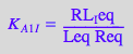
Correct relationship! It is four times more difficult to saturate the second site than the have the first one bound due to multiplicity of the binding sites.
3.2 Microscopic B-bidentateL model (bi-dentate ligand)
Mass balance
eq2_3_1_Bbidentate
![]()
Macroscopic steps
eq2_1_3_BmAcro
![]()
eq2_1_4_BmAcro

First ligand-binding step
eq2_3_4_Bbidentate:
solve(%, RL_Ieq):
%[1][1]:
eq3_2_1_Bbidentate:= RL_Ieq = %
![]()
eq2_3_5_Bbidentate:
solve(%, RL_I_Ieq):
%[1][1]:
eq3_2_2_Bbidentate:= RL_I_Ieq = %
![]()
eq2_3_7_Bbidentate:
solve(%, RL_b_ieq):
%[1][1]:
eq3_2_3_Bbidentate:= RL_b_ieq = %
![]()
Substitute into mass balance
eq2_3_1_Bbidentate:
% | eq3_2_3_Bbidentate | eq3_2_2_Bbidentate | eq3_2_1_Bbidentate:
eq3_2_4_Bbidentate:= %
![]()
Substitute into the macroscopic equation of the first step
eq2_1_3_BmAcro:
% | eq3_2_4_Bbidentate:
normal(%):
eq3_2_5_Bbidentate:= %
![]()
=> final equation
Second ligand-binding step
eq2_3_6_Bbidentate:
solve(%, RL_2eq):
%[1][1]:
eq3_2_6_Bbidentate:= RL_2eq = %
![]()
Substitute into the macroscopic equation for the second step
eq2_1_4_BmAcro:
% | eq3_2_6_Bbidentate | eq3_2_4_Bbidentate | eq3_2_1_Bbidentate:
normal(%):
eq3_2_7_Bbidentate:= %
![]()
=> final equation
Remove the first-step association constants (for convenience)
eq2_3_8_Bbidentate:
solve(%, K_A_1_I_I):
%[1]:
eq3_2_8_Bbidentate:= K_A_1_I_I = %
![]()
eq3_2_7_Bbidentate | eq3_2_8_Bbidentate:
normal(%):
eq3_2_9_Bbidentate:=%
![]()
=> final equation
Evaluate the same test situation: set individual binding constants to identical values
eq3_2_5_Bbidentate:
% | K_A_1_I = K | K_A_1_I_I = K
![]()
eq3_2_7_Bbidentate:
% | K_A_1_I = K | K_A_1_I_I = K | K_A_2_I_I = K:
normal(%)
![]()
=> Result makes perfect sence. The greater K_C_II is the more single-bound species with open second site is removed from binding of the second ligand; the smaller the second macroscopic association constant looks like!
Summary of general relationships between microscopic and macroscopic binding constants
===== Microscopic B model (mono-dentate ligand) ======
Binding of the first ligand:
eq3_1_4_Bmicro
![]()
Binding of the second ligand:
eq3_1_8_Bmicro
![]()
Binding of the second ligand in independent constants:
eq3_1_6_Bmicro
![]()
===== Microscopic B-bidentateL model (bi-dentate ligand) ======
Binding of the first ligand:
eq3_2_5_Bbidentate
![]()
Binding of the second ligand:
eq3_2_9_Bbidentate
![]()
Binding of the second ligand in independent constants:
eq3_2_7_Bbidentate
![]()
4. Derivation of equations for concentrations of species
I will prepare sets of equations separately for all three models.
4.1 Macroscopic B model
Goal: Express concentration of the free ligand, Leq, as a function of equilibrium constants and total concentrations.
Equations to use:
eq2_1_1_BmAcro
![]()
eq2_1_2_BmAcro
![]()
eq2_1_3_BmAcro
![]()
eq2_1_4_BmAcro
STEP 1: Express all R-containing species starting from the higher stoichiometry
Express RL_2eq out of the equilibrium constant equation
eq2_1_4_BmAcro:
solve(%, RL_2eq):
%[1][1]:
eq4_1_1_BmAcro:= RL_2eq = %
![]()
Express RLeq out of the equilibrium constant equation
eq2_1_3_BmAcro:
solve(%, RLeq):
%[1][1]:
eq4_1_2_BmAcro:= RLeq = %
![]()
STEP 2: Substitute all into mass balance for L and express Req
eq2_1_2_BmAcro:
% | eq4_1_1_BmAcro | eq4_1_2_BmAcro:
eq4_1_3_BmAcro:= %
![]()
solve(eq4_1_3_BmAcro,Req):
%[1][1]:
eq4_1_4_BmAcro:= Req = %
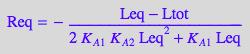
STEP 3: Substitute all into mass balance for R and attempt to solve for Leq
eq2_1_1_BmAcro :
% | eq4_1_1_BmAcro | eq4_1_2_BmAcro | eq4_1_4_BmAcro:
eq4_1_5_BmAcro:= %

=> This is an expression for numerical solution
Try to solve analytically
solve(eq4_1_5_BmAcro, Leq)
![]()
=> analytically insoluble; use numeric solution
4.2 Microscopic B model (mono-dentate binding only
Goal: Express concentration of the free ligand, Leq, as a function of equilibrium constants and total concentrations.
Equations to use:
eq2_2_1_Bmicro
![]()
eq2_2_2_Bmicro
![]()
eq2_2_3_Bmicro
![]()
eq2_2_4_Bmicro

eq2_2_5_Bmicro
eq2_2_6_Bmicro

STEP 1: Express all R-containing species starting from the higher stoichiometry
Express RL_2eq out of the equilibrium constant equation
eq2_2_6_Bmicro:
solve(%, RL_2eq):
%[1][1]:
eq4_2_1_Bmicro:= RL_2eq = %
![]()
Express RL_Ieq
eq2_2_4_Bmicro:
solve(%, RL_Ieq):
%[1][1]:
eq4_2_2_Bmicro:= RL_Ieq = %
![]()
Express RL_I_Ieq
eq2_2_5_Bmicro:
solve(%, RL_I_Ieq):
%[1][1]:
eq4_2_3_Bmicro:= RL_I_Ieq = %
![]()
STEP 2: Substitute all into mass balance for L and express Req
eq2_2_3_Bmicro:
% | eq4_2_1_Bmicro | eq2_2_1_Bmicro:
% | eq4_2_3_Bmicro | eq4_2_2_Bmicro:
solve(%, Req):
%[1][1]:
eq4_2_4_Bmicro:= Req = %
STEP 3: Substitute all into mass balance for R and attempt to solve for Leq
eq2_2_2_Bmicro:
% | eq2_2_1_Bmicro:
% | eq4_2_1_Bmicro | eq4_2_2_Bmicro | eq4_2_3_Bmicro | eq4_2_4_Bmicro:
eq4_2_5_Bmicro:= %
=> final equation for numeric solution
try to solve
solve(eq4_2_5_Bmicro, Leq)
![]()
=> insoluble. Use the numeric solution
4.3 Microscopic B-bidentateL model (bi-dentate ligand binding)
Goal: Express concentration of the free ligand, Leq, as a function of equilibrium constants and total concentrations.
Equations to use:
eq2_3_1_Bbidentate
![]()
eq2_3_2_Bbidentate
![]()
eq2_3_3_Bbidentate
![]()
eq2_3_4_Bbidentate

eq2_3_5_Bbidentate

eq2_3_6_Bbidentate
eq2_3_7_Bbidentate
STEP 1: Express all R-containing species starting from the higher stoichiometry
Express RL_2eq out of the equilibrium constant equation
eq2_3_6_Bbidentate:
solve(%, RL_2eq):
%[1][1]:
eq4_3_1_Bbidentate:= RL_2eq = %
![]()
Express RL_b_ieq
eq2_3_7_Bbidentate:
solve(%, RL_b_ieq):
%[1][1]:
eq4_3_2_Bbidentate:= RL_b_ieq = %
![]()
Express RL_Ieq
eq2_3_4_Bbidentate:
solve(%, RL_Ieq):
%[1][1]:
eq4_3_3_Bbidentate:= RL_Ieq = %
![]()
Express RL_I_Ieq
eq2_3_5_Bbidentate:
solve(%, RL_I_Ieq):
%[1][1]:
eq4_3_4_Bbidentate:= RL_I_Ieq = %
![]()
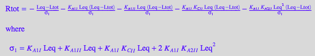
STEP 2: Substitute all into mass balance for L and express Req
eq2_3_3_Bbidentate;
% | eq2_3_1_Bbidentate;
% | eq4_3_1_Bbidentate | eq4_3_2_Bbidentate | eq4_3_3_Bbidentate | eq4_3_4_Bbidentate;
solve(%, Req):
%[1][1]:
eq4_3_5_Bbidentate:= Req = %
![]()
![]()
![]()
STEP 3: Substitute all into mass balance for R and attempt to solve for Leq
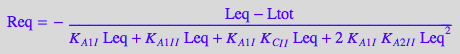
eq2_3_2_Bbidentate;
% | eq2_3_1_Bbidentate ;
% | eq4_3_1_Bbidentate | eq4_3_2_Bbidentate;
% | eq4_3_3_Bbidentate | eq4_3_4_Bbidentate;
% | eq4_3_5_Bbidentate;
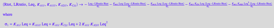
eq4_3_6_Bbidentate:= %
![]()
![]()
![]()
![]()

=> numeric solution
try to solve
S:=solve(eq4_3_6_Bbidentate, [Leq], Real)
![matrix([[Leq]]) in Dom::Interval(0, Ltot) intersect RootOf(K_A_1_I*K_A_2_I_I*z^3 + 2*K_A_1_I*K_A_2_I_I*Rtot*z^2 - K_A_1_I*K_A_2_I_I*Ltot*z^2 + K_A_1_I*K_C_I_I*z^2 + K_A_1_I_I*z^2 + K_A_1_I*z^2 - K_A_1_I*K_C_I_I*Ltot*z + K_A_1_I*K_C_I_I*Rtot*z - K_A_1_I_I*Ltot*z - K_A_1_I*Ltot*z + K_A_1_I_I*Rtot*z + K_A_1_I*Rtot*z + z - Ltot, z)](B_family_models_derivation_images/math140.png)
=> insoluble
Summary of equations for equilibrium concentrations of species
NOTE: Rename all equations for easier use.
===== Macroscopic B model ========
Expression for numeric solution for Leq:
eqRtot_BmAcro:=eq4_1_5_BmAcro

Expressions for other species
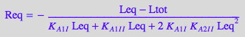
eqReq_BmAcro:=eq4_1_4_BmAcro
eqRLeq_BmAcro:=eq4_1_2_BmAcro
![]()
eqRL2eq_BmAcro:=eq4_1_1_BmAcro
![]()
====== Microscopic B model (mono-dentate binding only) =====
Expression for numeric solution for Leq:
eqRtot_Bmicro:=eq4_2_5_Bmicro
Expressions for other species
eqReq_Bmicro:=eq4_2_4_Bmicro
eqRLIIeq_Bmicro:=eq4_2_3_Bmicro
![]()
eqRLIeq_Bmicro:=eq4_2_2_Bmicro
![]()
eqRL2eq_Bmicro:=eq4_2_1_Bmicro
![]()
Expressions for dependent constants:
eqKA2I_Bmicro:=eq2_2_7_Bmicro
![]()
eqKB1_Bmicro:=eq2_2_8_Bmicro
![]()
===== Microscopic B-bidentateL model (bi-dentate ligand binding) =====
Expression for a numeric solution for Leq:
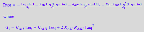
eqRtot_Bbidentate:=eq4_3_6_Bbidentate
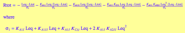
Other species:
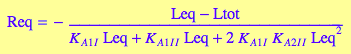
eqReq_Bbidentate:=eq4_3_5_Bbidentate
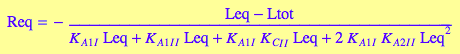
eqRLIIeq_Bbidentate:=eq4_3_4_Bbidentate
![]()
eqRLIeq_Bbidentate:=eq4_3_3_Bbidentate
![]()
eqRLbieq_Bbidentate:=eq4_3_2_Bbidentate
![]()
eqRL2eq_Bbidentate:=eq4_3_1_Bbidentate
![]()
Expressions for dependent constants:
eqKA2I_Bbidentate:=eq2_3_8_Bbidentate
![]()
eqKB1I_Bbidentate:=eq2_3_9_Bbidentate
![]()
eqKB2_Bbidentate:=eq2_3_10_Bbidentate
![]()
5. Prepare equations for a numeric solution
Introduce a convenient variable LRratio=Ltot/Rtot
eqLRratio:= Ltot = LRratio * Rtot
![]()
5.1 Macroscopic B model
STEP 1: Make a function for numeric solving of Rtot equation
fRtot_BmAcro:= (Rtot, LRratio, Leq, K_A_1, K_A_2) --> eqRtot_BmAcro[2] | eqLRratio;

Assume some constant values for testing
NOTE 1: Use different names for variables!!!
NOTE 2: Make sure the VALUES are all different and NOT just ORDER OF MAGNITUDS to make it easier for troubleshooting.
Rtot_value:=1e-3:
K_A_1_value:= 1e7:
K_A_2_value:= 1e8:
LR_ratio_max:= 2.5:
LR_ratio_value:= 0.8:
Leq_value:= 0.00000007373194321:
Test operation of the new function:
fRtot_BmAcro(Rtot_value, LR_ratio_value, Leq_value, K_A_1_value, K_A_2_value)
![]()
=> operational!
STEP 2: Define a procedure for numeric solving of this equation thus creating a function Leq=f(...)
/* WARNING: make sure the Leq search range starts with a non-zero number!!!!
* Use a number larger than that to create approximation of LRratio=0
*/
pnLeq_BmAcro:= proc(paramRtot, paramLRratio, paramK_A_1, paramK_A_2)
/* NOTE: Parameter names should be different from
variable names used in the equation!!!
If you see an error message:
"Error: Illegal operand [_index];
during evaluation of 'your function name'"
it means fsolve returned FAIL and you need to check
values of all parameters passed to the function fRtot
*/
local result;
begin
/* NOTE: Uncomment the strings below for debugging; comment out for normal operation.
* Display what was entered: */
//print(paramRtot, paramLRratio, paramK_A_1, paramK_A_2);
/* Numerically solving the equation for Leq in a restricted range.
* WARNING: make sure the range starts with a non-zero number!!!!
*/
result:=numeric::fsolve(
paramRtot - fRtot_BmAcro(paramRtot, paramLRratio, paramLeq, paramK_A_1, paramK_A_2),
paramLeq=10e-32..paramRtot*paramLRratio);
/* See the full result */
//print(result);
/* extract answer from equation */
result[1][2]
end_proc;
![]()
Test operation:
pnLeq_BmAcro(Rtot_value, LR_ratio_value, K_A_1_value, K_A_2_value)
![]()
STEP 3: Define functions for equilibrium concentrations of all species
(begin with listing equations for the species)
Expressions for other species:
Req
eqReq_BmAcro;
pnReq_BmAcro:= proc(paramRtot, paramLRratio, paramK_A_1, paramK_A_2)
local L;
begin
L:=pnLeq_BmAcro(paramRtot, paramLRratio, paramK_A_1, paramK_A_2);
// Insert equation for this species and substitute all parameters
eqReq_BmAcro[2] | Ltot=paramLRratio*paramRtot | Leq=L | K_A_1=paramK_A_1 | K_A_2=paramK_A_2;
end_proc

![]()
test
pnReq_BmAcro(Rtot_value, LR_ratio_value, K_A_1_value, K_A_2_value);
![]()
=>operational
RLeq
eqRLeq_BmAcro;
pnRLeq_BmAcro:= proc(paramRtot, paramLRratio, paramK_A_1, paramK_A_2)
local L, R;
begin
L:=pnLeq_BmAcro(paramRtot, paramLRratio, paramK_A_1, paramK_A_2);
R:=pnReq_BmAcro(paramRtot, paramLRratio, paramK_A_1, paramK_A_2);
// Insert equation for this species and substitute all parameters
eqRLeq_BmAcro[2] | Leq=L | Req=R | K_A_1=paramK_A_1 ;
end_proc
![]()
![]()
Test
pnRLeq_BmAcro(Rtot_value, LR_ratio_value, K_A_1_value, K_A_2_value);
![]()
=> operational
eqRL2eq_BmAcro;
pnRL2eq_BmAcro:= proc(paramRtot, paramLRratio, paramK_A_1, paramK_A_2)
local L, RL;
begin
L:=pnLeq_BmAcro(paramRtot, paramLRratio, paramK_A_1, paramK_A_2);
RL:=pnRLeq_BmAcro(paramRtot, paramLRratio, paramK_A_1, paramK_A_2);
// Insert equation for this species and substitute all parameters
eqRL2eq_BmAcro[2] | Leq=L | RLeq=RL | K_A_2=paramK_A_2;
end_proc
![]()
![]()
Test
pnRL2eq_BmAcro(Rtot_value, LR_ratio_value, K_A_1_value, K_A_2_value);
![]()
=> operational
STEP 4: Catch errors in substitution of equations (cut-and-paste glitches)
Collect all the test lines and re-run. Make sure all numbers come out different.
Cut-and-paste glitches come out as identical numbers.
pnLeq_BmAcro(Rtot_value, LR_ratio_value, K_A_1_value, K_A_2_value);
pnReq_BmAcro(Rtot_value, LR_ratio_value, K_A_1_value, K_A_2_value);
pnRLeq_BmAcro(Rtot_value, LR_ratio_value, K_A_1_value, K_A_2_value);
pnRL2eq_BmAcro(Rtot_value, LR_ratio_value, K_A_1_value, K_A_2_value);
![]()
![]()
![]()
![]()
=> All different! No cut-and-paste typos.
STEP 5: Collect all these names in Section 6 for saving on the disk.
5.2 Microscopic B model (mono-dentate binding only)
STEP 1: Make a function for numeric solving of Rtot equation
eqRtot_Bmicro:
fRtot_Bmicro:= (Rtot, LRratio, Leq, K_A_1_I, K_A_1_I_I, K_A_2_I_I) --> eqRtot_Bmicro[2] | eqLRratio;
Assume new constants
NOTE 1: Use different names for variables!!!
NOTE 2: Make sure the VALUES are all different and NOT just ORDER OF MAGNITUDS to make it easier for troubleshooting.
K_A_1_I_value:=1e4:
K_A_1_I_I_value:=1e6:
K_A_2_I_I_value:=1e5:
Leq_value:=0.0000001890503389: // taken from test of the procedure (below)
Test
fRtot_Bmicro(Rtot_value, LR_ratio_value, Leq_value, K_A_1_I_value, K_A_1_I_I_value, K_A_2_I_I_value)
![]()
=> operational
STEP 2: Define a procedure for numeric solving of this equation thus creating a function Leq=f(...)
/* WARNING: make sure the Leq search range starts with a non-zero number!!!!
* Use a number larger than that to create approximation of LRratio=0
*/
pnLeq_Bmicro:= proc(paramRtot, paramLRratio, paramK_A_1_I, paramK_A_1_I_I, paramK_A_2_I_I)
/* NOTE: Parameter names should be different from
variable names used in the equation!!!
If you see an error message:
"Error: Illegal operand [_index];
during evaluation of 'your function name'"
it means fsolve returned FAIL and you need to check
values of all parameters passed to the function fRtot
*/
local result;
begin
/* NOTE: Uncomment the strings below for debugging; comment out for normal operation.
* Display what was entered: */
//print(paramRtot, paramLRratio, paramK_A_1_I, paramK_A_1_I_I, paramK_A_2_I_I);
/* Numerically solving the equation for Leq in a restricted range.
* WARNING: make sure the range starts with a non-zero number!!!!
*/
result:=numeric::fsolve(
paramRtot - fRtot_Bmicro(paramRtot, paramLRratio, paramLeq, paramK_A_1_I, paramK_A_1_I_I, paramK_A_2_I_I),
paramLeq=10e-32..paramRtot*paramLRratio);
/* See the full result */
//print(result);
/* extract answer from equation */
result[1][2]
end_proc;
![]()
test
pnLeq_Bmicro(Rtot_value, LR_ratio_value, K_A_1_I_value, K_A_1_I_I_value, K_A_2_I_I_value)
![]()
=> operational
STEP 3: Define functions for equilibrium concentrations of all species
(begin with listing equations for the species)
Expressions for other species:
Req
eqReq_Bmicro;
pnReq_Bmicro:= proc(paramRtot, paramLRratio, paramK_A_1_I, paramK_A_1_I_I, paramK_A_2_I_I)
local L;
begin
L:=pnLeq_Bmicro(paramRtot, paramLRratio, paramK_A_1_I, paramK_A_1_I_I, paramK_A_2_I_I);
// Insert equation for this species and substitute all parameters
eqReq_Bmicro[2] | Ltot=paramLRratio*paramRtot | Leq=L | K_A_1_I=paramK_A_1_I | K_A_1_I_I=paramK_A_1_I_I | K_A_2_I_I=paramK_A_2_I_I ;
end_proc

![]()
test
pnReq_Bmicro(Rtot_value, LR_ratio_value, K_A_1_I_value, K_A_1_I_I_value, K_A_2_I_I_value)
![]()
RLIIeq
eqRLIIeq_Bmicro;
pnRLIIeq_Bmicro:= proc(paramRtot, paramLRratio, paramK_A_1_I, paramK_A_1_I_I, paramK_A_2_I_I)
local L, R;
begin
L:=pnLeq_Bmicro(paramRtot, paramLRratio, paramK_A_1_I, paramK_A_1_I_I, paramK_A_2_I_I);
R:=pnReq_Bmicro(paramRtot, paramLRratio, paramK_A_1_I, paramK_A_1_I_I, paramK_A_2_I_I);
// Insert equation for this species and substitute all parameters
eqRLIIeq_Bmicro[2] | Ltot=paramLRratio*paramRtot | Leq=L | Req=R | K_A_1_I=paramK_A_1_I | K_A_1_I_I=paramK_A_1_I_I | K_A_2_I_I=paramK_A_2_I_I ;
end_proc
![]()
![]()
test
pnRLIIeq_Bmicro(Rtot_value, LR_ratio_value, K_A_1_I_value, K_A_1_I_I_value, K_A_2_I_I_value)
![]()
=> operational
RLIeq
eqRLIeq_Bmicro;
pnRLIeq_Bmicro:= proc(paramRtot, paramLRratio, paramK_A_1_I, paramK_A_1_I_I, paramK_A_2_I_I)
local L, R;
begin
L:=pnLeq_Bmicro(paramRtot, paramLRratio, paramK_A_1_I, paramK_A_1_I_I, paramK_A_2_I_I);
R:=pnReq_Bmicro(paramRtot, paramLRratio, paramK_A_1_I, paramK_A_1_I_I, paramK_A_2_I_I);
// Insert equation for this species and substitute all parameters
eqRLIeq_Bmicro[2] | Ltot=paramLRratio*paramRtot | Leq=L | Req=R | K_A_1_I=paramK_A_1_I | K_A_1_I_I=paramK_A_1_I_I | K_A_2_I_I=paramK_A_2_I_I ;
end_proc
![]()
![]()
test
pnRLIeq_Bmicro(Rtot_value, LR_ratio_value, K_A_1_I_value, K_A_1_I_I_value, K_A_2_I_I_value)
![]()
RL2eq
eqRL2eq_Bmicro;
pnRL2eq_Bmicro:= proc(paramRtot, paramLRratio, paramK_A_1_I, paramK_A_1_I_I, paramK_A_2_I_I)
local L, RLI;
begin
L:=pnLeq_Bmicro(paramRtot, paramLRratio, paramK_A_1_I, paramK_A_1_I_I, paramK_A_2_I_I);
RLI:=pnRLIeq_Bmicro(paramRtot, paramLRratio, paramK_A_1_I, paramK_A_1_I_I, paramK_A_2_I_I);
// Insert equation for this species and substitute all parameters
eqRL2eq_Bmicro[2] | Ltot=paramLRratio*paramRtot | Leq=L | RL_Ieq=RLI | K_A_1_I=paramK_A_1_I | K_A_1_I_I=paramK_A_1_I_I | K_A_2_I_I=paramK_A_2_I_I ;
end_proc
![]()
![]()
test
pnRL2eq_Bmicro(Rtot_value, LR_ratio_value, K_A_1_I_value, K_A_1_I_I_value, K_A_2_I_I_value)
![]()
=> operational
STEP 4: Catch errors in substitution of equations (cut-and-paste glitches)
Collect all the test lines and re-run. Make sure all numbers come out different.
Cut-and-paste glitches come out as identical numbers.
pnLeq_Bmicro(Rtot_value, LR_ratio_value, K_A_1_I_value, K_A_1_I_I_value, K_A_2_I_I_value);
pnReq_Bmicro(Rtot_value, LR_ratio_value, K_A_1_I_value, K_A_1_I_I_value, K_A_2_I_I_value);
pnRLIIeq_Bmicro(Rtot_value, LR_ratio_value, K_A_1_I_value, K_A_1_I_I_value, K_A_2_I_I_value);
pnRLIeq_Bmicro(Rtot_value, LR_ratio_value, K_A_1_I_value, K_A_1_I_I_value, K_A_2_I_I_value);
pnRL2eq_Bmicro(Rtot_value, LR_ratio_value, K_A_1_I_value, K_A_1_I_I_value, K_A_2_I_I_value);
![]()
![]()
![]()
![]()
![]()
=> all different! Good. No cut-and-paste typos.
STEP 5: Collect all these names in Section 6 for saving on the disk.
5.3 Microscopic B-bidentatateL model (bi-dentate ligand)
STEP 1: Make a function for numeric solving of Rtot equation
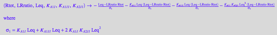
fRtot_Bbidentate:= (Rtot, LRratio, Leq, K_A_1_I, K_A_1_I_I, K_A_2_I_I, K_C_I_I) --> eqRtot_Bbidentate[2] | eqLRratio;
Assume new constants
NOTE 1: Use different names for variables!!!
NOTE 2: Make sure the VALUES are all different and NOT just ORDER OF MAGNITUDS to make it easier for troubleshooting.
Rtot_value:=1e-3:
LR_ratio_value:= 0.5:
K_A_1_I_value:=2e4:
K_A_1_I_I_value:=1e2:
K_A_2_I_I_value:=3e5:
K_C_I_I_value:=11:
test
fRtot_Bbidentate(Rtot_value, LR_ratio_value, Leq_value, K_A_1_I_value, K_A_1_I_I_value, K_A_2_I_I_value, K_C_I_I_value)
![]()
=> operational
STEP 2: Define a procedure for numeric solving of this equation thus creating a function Leq=f(...)
/* WARNING: make sure the Leq search range starts with a non-zero number!!!!
* Use a number larger than that to create approximation of LRratio=0
*/
pnLeq_Bbidentate:= proc(paramRtot, paramLRratio, paramK_A_1_I, paramK_A_1_I_I, paramK_A_2_I_I, paramK_C_I_I)
/* NOTE: Parameter names should be different from
variable names used in the equation!!!
If you see an error message:
"Error: Illegal operand [_index];
during evaluation of 'your function name'"
it means fsolve returned FAIL and you need to check
values of all parameters passed to the function fRtot
*/
local result;
begin
/* NOTE: Uncomment the strings below for debugging; comment out for normal operation.
* Display what was entered: */
//print(paramRtot, paramLRratio, paramK_A_1_I, paramK_A_1_I_I, paramK_A_2_I_I, paramK_C_I_I);
/* Numerically solving the equation for Leq in a restricted range.
* WARNING: make sure the range starts with a non-zero number!!!!
*/
result:=numeric::fsolve(
paramRtot - fRtot_Bbidentate(paramRtot, paramLRratio, paramLeq, paramK_A_1_I, paramK_A_1_I_I, paramK_A_2_I_I, paramK_C_I_I),
paramLeq=10e-32..paramRtot*paramLRratio);
/* See the full result */
//print(result);
/* extract answer from equation */
result[1][2]
end_proc;
![]()
test
pnLeq_Bbidentate(Rtot_value, LR_ratio_value, K_A_1_I_value, K_A_1_I_I_value, K_A_2_I_I_value, K_C_I_I_value)
![]()
STEP 3: Define functions for equilibrium concentrations of all species
(begin with listing equations for the species)
Expressions for other species:
Req
eqReq_Bbidentate;
pnReq_Bbidentate:= proc(paramRtot, paramLRratio, paramK_A_1_I, paramK_A_1_I_I, paramK_A_2_I_I, paramK_C_I_I)
local L;
begin
L:=pnLeq_Bbidentate(paramRtot, paramLRratio, paramK_A_1_I, paramK_A_1_I_I, paramK_A_2_I_I, paramK_C_I_I);
// Insert equation for this species and substitute all parameters
eqReq_Bbidentate[2] | Ltot=paramLRratio*paramRtot | Leq=L | K_A_1_I=paramK_A_1_I | K_A_1_I_I=paramK_A_1_I_I | K_A_2_I_I=paramK_A_2_I_I | K_C_I_I=paramK_C_I_I;
end_proc

![]()
test
pnReq_Bbidentate(Rtot_value, LR_ratio_value, K_A_1_I_value, K_A_1_I_I_value, K_A_2_I_I_value, K_C_I_I_value)
![]()
RLIeq
eqRLIeq_Bbidentate;
pnRLIeq_Bbidentate:= proc(paramRtot, paramLRratio, paramK_A_1_I, paramK_A_1_I_I, paramK_A_2_I_I, paramK_C_I_I)
local L, R;
begin
L:=pnLeq_Bbidentate(paramRtot, paramLRratio, paramK_A_1_I, paramK_A_1_I_I, paramK_A_2_I_I, paramK_C_I_I);
R:=pnReq_Bbidentate(paramRtot, paramLRratio, paramK_A_1_I, paramK_A_1_I_I, paramK_A_2_I_I, paramK_C_I_I);
// Insert equation for this species and substitute all parameters
eqRLIeq_Bbidentate[2] | Ltot=paramLRratio*paramRtot | Leq=L | Req=R | K_A_1_I=paramK_A_1_I | K_A_1_I_I=paramK_A_1_I_I | K_A_2_I_I=paramK_A_2_I_I | K_C_I_I=paramK_C_I_I;
end_proc
![]()
![]()
test
pnRLIeq_Bbidentate(Rtot_value, LR_ratio_value, K_A_1_I_value, K_A_1_I_I_value, K_A_2_I_I_value, K_C_I_I_value)
![]()
RLIIeq
eqRLIIeq_Bbidentate;
pnRLIIeq_Bbidentate:= proc(paramRtot, paramLRratio, paramK_A_1_I, paramK_A_1_I_I, paramK_A_2_I_I, paramK_C_I_I)
local L, R;
begin
L:=pnLeq_Bbidentate(paramRtot, paramLRratio, paramK_A_1_I, paramK_A_1_I_I, paramK_A_2_I_I, paramK_C_I_I);
R:=pnReq_Bbidentate(paramRtot, paramLRratio, paramK_A_1_I, paramK_A_1_I_I, paramK_A_2_I_I, paramK_C_I_I);
// Insert equation for this species and substitute all parameters
eqRLIIeq_Bbidentate[2] | Ltot=paramLRratio*paramRtot | Leq=L | Req=R | K_A_1_I=paramK_A_1_I | K_A_1_I_I=paramK_A_1_I_I | K_A_2_I_I=paramK_A_2_I_I | K_C_I_I=paramK_C_I_I;
end_proc
![]()
![]()
test
pnRLIIeq_Bbidentate(Rtot_value, LR_ratio_value, K_A_1_I_value, K_A_1_I_I_value, K_A_2_I_I_value, K_C_I_I_value)
![]()
RLbieq
eqRLbieq_Bbidentate;
pnRLbieq_Bbidentate:= proc(paramRtot, paramLRratio, paramK_A_1_I, paramK_A_1_I_I, paramK_A_2_I_I, paramK_C_I_I)
local L, RLI;
begin
L:=pnLeq_Bbidentate(paramRtot, paramLRratio, paramK_A_1_I, paramK_A_1_I_I, paramK_A_2_I_I, paramK_C_I_I);
RLI:=pnRLIeq_Bbidentate(paramRtot, paramLRratio, paramK_A_1_I, paramK_A_1_I_I, paramK_A_2_I_I, paramK_C_I_I);
// Insert equation for this species and substitute all parameters
eqRLbieq_Bbidentate[2] | Ltot=paramLRratio*paramRtot | Leq=L | RL_Ieq=RLI | K_A_1_I=paramK_A_1_I | K_A_1_I_I=paramK_A_1_I_I | K_A_2_I_I=paramK_A_2_I_I | K_C_I_I=paramK_C_I_I;
end_proc
![]()
![]()
test
pnRLbieq_Bbidentate(Rtot_value, LR_ratio_value, K_A_1_I_value, K_A_1_I_I_value, K_A_2_I_I_value, K_C_I_I_value)
![]()
RL2eq
eqRL2eq_Bbidentate;
pnRL2eq_Bbidentate:= proc(paramRtot, paramLRratio, paramK_A_1_I, paramK_A_1_I_I, paramK_A_2_I_I, paramK_C_I_I)
local L, RLI;
begin
L:=pnLeq_Bbidentate(paramRtot, paramLRratio, paramK_A_1_I, paramK_A_1_I_I, paramK_A_2_I_I, paramK_C_I_I);
RLI:=pnRLIeq_Bbidentate(paramRtot, paramLRratio, paramK_A_1_I, paramK_A_1_I_I, paramK_A_2_I_I, paramK_C_I_I);
// Insert equation for this species and substitute all parameters
eqRL2eq_Bbidentate[2] | Ltot=paramLRratio*paramRtot | Leq=L | RL_Ieq=RLI | K_A_1_I=paramK_A_1_I | K_A_1_I_I=paramK_A_1_I_I | K_A_2_I_I=paramK_A_2_I_I | K_C_I_I=paramK_C_I_I;
end_proc
![]()
![]()
test
pnRL2eq_Bbidentate(Rtot_value, LR_ratio_value, K_A_1_I_value, K_A_1_I_I_value, K_A_2_I_I_value, K_C_I_I_value)
![]()
STEP 4: Catch errors in substitution of equations (cut-and-paste glitches)
Collect all the test lines and re-run. Make sure all numbers come out different.
Cut-and-paste glitches come out as identical numbers.
pnLeq_Bbidentate(Rtot_value, LR_ratio_value, K_A_1_I_value, K_A_1_I_I_value, K_A_2_I_I_value, K_C_I_I_value);
pnReq_Bbidentate(Rtot_value, LR_ratio_value, K_A_1_I_value, K_A_1_I_I_value, K_A_2_I_I_value, K_C_I_I_value);
pnRLIeq_Bbidentate(Rtot_value, LR_ratio_value, K_A_1_I_value, K_A_1_I_I_value, K_A_2_I_I_value, K_C_I_I_value);
pnRLIIeq_Bbidentate(Rtot_value, LR_ratio_value, K_A_1_I_value, K_A_1_I_I_value, K_A_2_I_I_value, K_C_I_I_value);
pnRLbieq_Bbidentate(Rtot_value, LR_ratio_value, K_A_1_I_value, K_A_1_I_I_value, K_A_2_I_I_value, K_C_I_I_value);
pnRL2eq_Bbidentate(Rtot_value, LR_ratio_value, K_A_1_I_value, K_A_1_I_I_value, K_A_2_I_I_value, K_C_I_I_value);
![]()
![]()
![]()
![]()
![]()
![]()
=> all different. OK
STEP 5: Collect all these names in Section 6 for saving on the disk.
6. Save results on disk for future use
(you can retrieve them later by executing: fread(filename,Quiet))
ProjectName;
CurrentPath
![]()
![]()
Save all numeric solutions:
filename:=CurrentPath.ProjectName.".mb";
write(filename,
// Macroscopic B model
// - equations
eqRtot_BmAcro,
eqReq_BmAcro,
eqRLeq_BmAcro,
eqRL2eq_BmAcro,
// - procedures
fRtot_BmAcro,
pnLeq_BmAcro,
pnReq_BmAcro,
pnRLeq_BmAcro,
pnRL2eq_BmAcro,
// Microscopic B model (mono-dentate binding only)
// - equations
eqRtot_Bmicro,
eqReq_Bmicro,
eqRLIIeq_Bmicro,
eqRLIeq_Bmicro,
eqRL2eq_Bmicro,
// - dependent constants
eqKA2I_Bmicro,
eqKB1_Bmicro,
// - procedures
fRtot_Bmicro,
pnLeq_Bmicro,
pnReq_Bmicro,
pnRLIIeq_Bmicro,
pnRLIeq_Bmicro,
pnRL2eq_Bmicro,
// Microscopic B-bidentateL model (bi-dentate ligand)
// - equations
eqRtot_Bbidentate,
eqReq_Bbidentate,
eqRLIIeq_Bbidentate,
eqRLIeq_Bbidentate,
eqRLbieq_Bbidentate,
eqRL2eq_Bbidentate,
// - dependent contants
eqKA2I_Bbidentate,
eqKB1I_Bbidentate,
eqKB2_Bbidentate,
// - procedures
fRtot_Bbidentate,
pnLeq_Bbidentate,
pnReq_Bbidentate,
pnRLIeq_Bbidentate,
pnRLIIeq_Bbidentate,
pnRLbieq_Bbidentate,
pnRL2eq_Bbidentate
)

Conclusions
Derivation of all three models have been completed. All three checked out correctly in the next (analysis) step. Ready for implementation in IDAP.