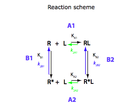
Analysis U-R-RL model
Binding of one ligand coupled with intramolecular isomerization
(this is the same model as ABC1, just in a new notation)
4. Summary of some graphical results
6. Reproduce a graph for equilibrium concentrations using a numeric solution
7. Save results on disk for future use
In this notebook I will re-analyze U-R-RL model using derivations performed in
EKM16.Analysis_of_multistep_kinetic_mechanisms/Equilibria/LRIM_U_R_RL.derivation.mn
clean up workspace
reset()
Set path to save results into:
ProjectName:="U_R_RL";
CurrentPath:="/Users/kovrigin/Documents/Workspace/Data/Data.XV/EKM16.Analysis_of_multistep_kinetic_mechanisms/Equilibria/";
![]()
![]()
Read results of derivations
filename:=CurrentPath.ProjectName.".mb";
fread(filename,Quiet):
![]()
Display equations (change : for ; to see the equation. Makes Mupad slow if all shown)
Leq_U_R_RL:
Req_U_R_RL:
RLeq_U_R_RL:;
Rstareq_U_R_RL:;
RstarLeq_U_R_RL:;
KA2_U_R_RL:;
Display functions
fLeq_U_R_RL:
fReq_U_R_RL:
fRLeq_U_R_RL:
fRstareq_U_R_RL:
fRstarLeq_U_R_RL:
Equation for a numerical solution
Rtot_U_R_RL

Set some realistic values for constants:
Total_R:=1e-3;
Total_L:=0.5e-3;
Ka1:=1e7;
Kb1:=2/1;
Kb2:=0.1;
LRratio_max:=1.2;
![]()
![]()
![]()
![]()
![]()
![]()
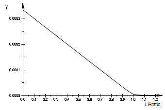
[R]
pReq:= plot::Function2d(
Function=(fReq_U_R_RL(Total_R, Total_R*LRratio, Ka1, Kb1, Kb2)),
LegendText="[R]",
Color = RGB::Black,
XMin=(0),
XMax=(LRratio_max),
XName=(LRratio),
TitlePositionX=(0)):
plot(pReq)
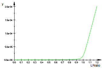
[L]
pLeq:= plot::Function2d(
Function=(fLeq_U_R_RL(Total_R, Total_R*LRratio, Ka1, Kb1, Kb2)),
LegendText="[L]",
Color = RGB::Green,
XMin=(0),
XMax=(LRratio_max),
XName=(LRratio),
TitlePositionX=(0)):
plot(pLeq)
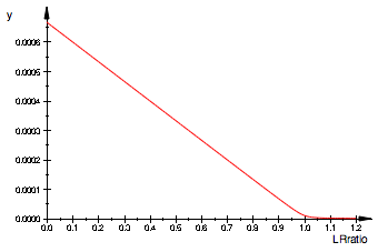
[R*]
pRstareq:= plot::Function2d(
Function=(fRstareq_U_R_RL(Total_R, Total_R*LRratio, Ka1, Kb1, Kb2)),
LegendText="[R*]",
Color = RGB::Red,
XMin=(0),
XMax=(LRratio_max),
XName=(LRratio),
TitlePositionX=(0)):
plot(pRstareq)
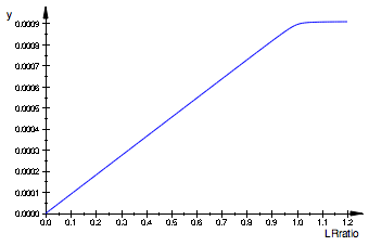
[RL]
pRLeq:= plot::Function2d(
Function=(fRLeq_U_R_RL(Total_R, Total_R*LRratio, Ka1, Kb1, Kb2)),
LegendText="[RL]",
Color = RGB::Blue,
XMin=(0),
XMax=(LRratio_max),
XName=(LRratio),
TitlePositionX=(0)):
plot(pRLeq)
[R*L]
pRstarLeq:= plot::Function2d(
Function=(fRstarLeq_U_R_RL(Total_R, Total_R*LRratio, Ka1, Kb1, Kb2)),
LegendText="[R*L]",
Color = RGB::Magenta,
XMin=(0),
XMax=(LRratio_max),
XName=(LRratio),
TitlePositionX=(0)):
plot(pRstarLeq)
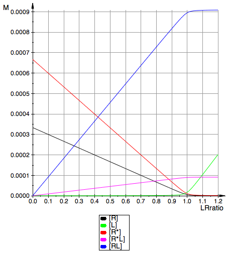
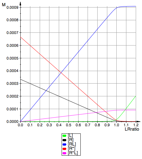
Plot all on one graph
plot(pReq, pLeq, pRstareq, pRstarLeq, pRLeq, YAxisTitle="M",
Height=180, Width=160,TicksLabelFont=["Helvetica",12,[0,0,0],Left],
AxesTitleFont=["Helvetica",14,[0,0,0],Left],
XGridVisible=TRUE, YGridVisible=TRUE,
LegendVisible=TRUE, LegendFont=["Helvetica",14,[0,0,0],Left]);
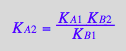
Compute dependent constant
KA2_U_R_RL ;
% | K_A_1=Ka1 | K_B_1=Kb1 | K_B_2=Kb2;
log(10,%[2])

![]()
![]()
`
Equations behave as expected.
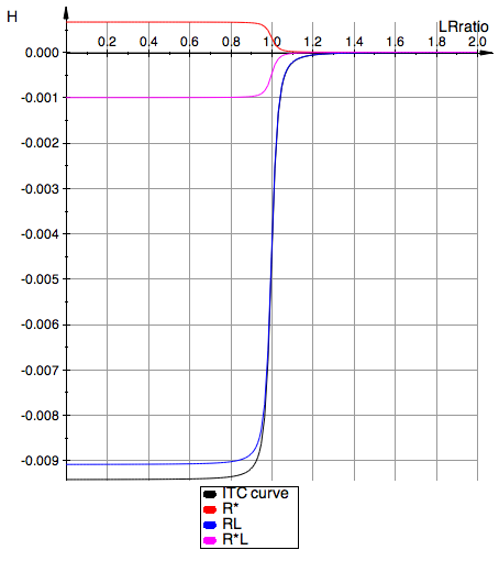
I would like to simulate what ITC curve should look like for this system
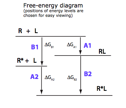
Set enthalpies for formation of 1 mole of each species.
in units kJ/mol relatively to R. Use free-energy diagram as a guide b/c enthalpy diagram will be similar.
Use pretty arbitrary values
H_R:=0:
H_Rstar:=-1:
H_RL:=-10:
H_RstarL:=-11:
LRratio_max:=2:
Heat of titration is a derivative of all concentration of species times corresponding enthalpies.
Define derivatives:
f_Rstar:=(Rtot, LRratio, K_A_1, K_B_1, K_B_2) --> fRstareq_U_R_RL(Rtot, Rtot*LRratio, K_A_1, K_B_1, K_B_2):
df_Rstar:=(Rtot, LRratio, K_A_1, K_B_1, K_B_2) --> diff(f_Rstar(Rtot, LRratio, K_A_1, K_B_1, K_B_2),LRratio):
f_RL:=(Rtot, LRratio, K_A_1, K_B_1, K_B_2) --> fRLeq_U_R_RL(Rtot, Rtot*LRratio, K_A_1, K_B_1, K_B_2):
df_RL:=(Rtot, LRratio, K_A_1, K_B_1, K_B_2) --> diff(f_RL(Rtot, LRratio, K_A_1, K_B_1, K_B_2),LRratio):
f_RstarL:=(Rtot, LRratio, K_A_1, K_B_1, K_B_2) --> fRstarLeq_U_R_RL(Rtot, Rtot*LRratio, K_A_1, K_B_1, K_B_2):
df_RstarL:=(Rtot, LRratio, K_A_1, K_B_1, K_B_2) --> diff(f_RstarL(Rtot, LRratio, K_A_1, K_B_1, K_B_2),LRratio):
Prepare plots of individual contributions and summed
R*
pRstar_ITC:= plot::Function2d(
Function=(H_Rstar*df_Rstar(Total_R, LRratio, Ka1, Kb1, Kb2)),
LegendText="R*",
Color = RGB::Red,
XMin=(0),
XMax=(LRratio_max),
XName=(LRratio),
TitlePositionX=(0)):
plot(pRstar_ITC);
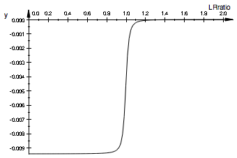
RL
pRL_ITC:= plot::Function2d(
Function=(H_RL*df_RL(Total_R, LRratio, Ka1, Kb1, Kb2)),
LegendText="RL",
Color = RGB::Blue,
XMin=(0),
XMax=(LRratio_max),
XName=(LRratio),
TitlePositionX=(0)):
plot(pRL_ITC);
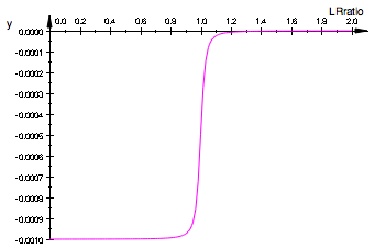
R*L
pRstarL_ITC:= plot::Function2d(
Function=(H_RstarL*df_RstarL(Total_R, LRratio, Ka1, Kb1, Kb2)),
LegendText="R*L",
Color = RGB::Magenta,
XMin=(0),
XMax=(LRratio_max),
XName=(LRratio),
TitlePositionX=(0)):
plot(pRstarL_ITC);
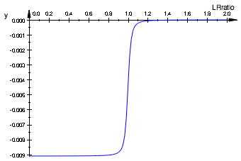
A sum of all
pSum_ITC:= plot::Function2d(
Function=(H_Rstar * df_Rstar(Total_R, LRratio, Ka1, Kb1, Kb2) +
H_RL * df_RL(Total_R, LRratio, Ka1, Kb1, Kb2) +
H_RstarL * df_RstarL(Total_R, LRratio, Ka1, Kb1, Kb2)
),
LegendText="ITC curve",
Color = RGB::Black,
XMin=(0),
XMax=(LRratio_max),
XName=(LRratio),
TitlePositionX=(0)):
plot(pSum_ITC);
Plot all on one graph
plot(pSum_ITC, pRstar_ITC, pRL_ITC, pRstarL_ITC, YAxisTitle="H",
Height=180, Width=160,TicksLabelFont=["Helvetica",12,[0,0,0],Left],
AxesTitleFont=["Helvetica",14,[0,0,0],Left],
XGridVisible=TRUE, YGridVisible=TRUE,
LegendVisible=TRUE, LegendFont=["Helvetica",14,[0,0,0],Left]);

Simple test results
|
Total_R:=1e-3; Total_L:=0.5e-3; Ka1:=1e7; Kb1:=2/1; Kb2:=0.1; LRratio_max:=1.2; |
|
|
H_R:=0: H_Rstar:=-1: H_RL:=-10: H_RstarL:=-11:
LRratio_max:=2: |
|
Equation for numerical solution
Rtot_U_R_RL

Make a function and switch to LRratio=
fRtot:=(Rtot, LRratio, Leq, K_A_1, K_B_1, K_B_2) --> Rtot_U_R_RL[2] | Ltot=Rtot*LRratio

Assume some constant values
Total_R:=1e-3:
Total_L:=0.5e-3:
Ka1:=1e7:
Kb1:=2/1:
Kb2:=0.1:
LRratio_max:=1.2:
Define a procedure for numeric solving the equation Rtot=f([L]) for [L] essentially creating a function [L]=f(Rtot,...)
// WARNING: make sure the Leq search range starts with a non-zero number!!!!
pnLeq:= proc(Total_R, LRratio, Ka1, Kb1, Kb2)
// Parameter names should be different from
// variable names used in the equation!!!
begin
// numeric solving equation for Leq in a restricted range.
// WARNING: make sure the range starts with a non-zero number!!!!
result:=numeric::fsolve(Total_R-fRtot(Total_R, LRratio, Leq, Ka1, Kb1, Kb2),Leq=10e-32..Total_R*LRratio);
// extract answer from equation
result[1][2]
end_proc;
![]()
DIGITS:=10;
pnLeq(Total_R, 0.5, Ka1, Kb1, Kb2)
![]()
![]()
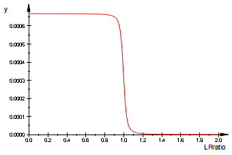
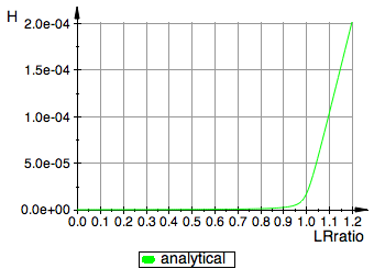
Test versus analytical solution
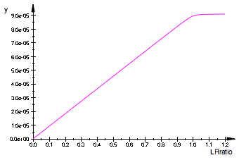
[L]
For plotting: add a wrapper function with a single argument
// add wrapper function :
fnLeq:=LRratio -> pnLeq(Total_R, LRratio, Ka1, Kb1, Kb2);
// plot analytical solution
Leq_analytical:= plot::Function2d(
Function=(fLeq_U_R_RL(Total_R, Total_R*LRratio, Ka1, Kb1, Kb2)),
LegendText="analytical",
Color = RGB::Green,
XMin=(0),
XMax=(LRratio_max),
XName=(LRratio),
TitlePositionX=(0)):
plot(Leq_analytical, YAxisTitle="H",
Height=90, Width=120,TicksLabelFont=["Helvetica",12,[0,0,0],Left],
AxesTitleFont=["Helvetica",14,[0,0,0],Left],
XGridVisible=TRUE, YGridVisible=TRUE,
LegendVisible=TRUE, LegendFont=["Helvetica",14,[0,0,0],Left]);
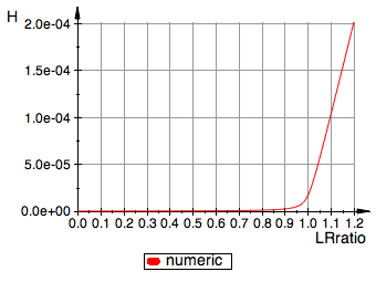
// plot numeric solution on top
Leq_numeric:= plot::Function2d(
Function=(fnLeq),
LegendText="numeric",
Color = RGB::Red,
XMin=(0),
XMax=(LRratio_max),
XName=(LRratio),
TitlePositionX=(0)):
plot(Leq_numeric, YAxisTitle="H",
Height=90, Width=120,TicksLabelFont=["Helvetica",12,[0,0,0],Left],
AxesTitleFont=["Helvetica",14,[0,0,0],Left],
XGridVisible=TRUE, YGridVisible=TRUE,
LegendVisible=TRUE, LegendFont=["Helvetica",14,[0,0,0],Left]);

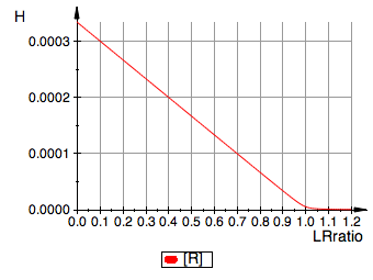
6. Reproduce a graph for equilibrium concentrations using a numeric solution
Copy-paste over the equations for equilibrium concentrations from Equilibria/U_R_RL_derivation.mn
(source equation number)
Dependent constant
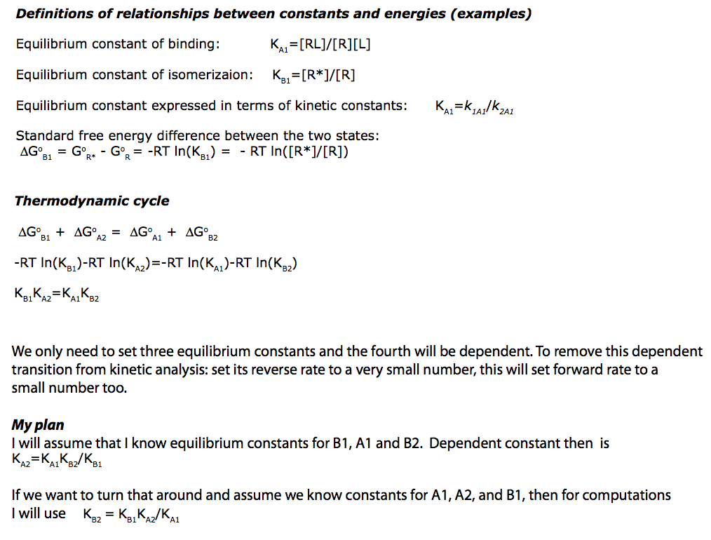
eq6_0:= K_A_2 = K_A_1*K_B_2 / K_B_1
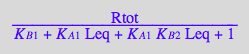
[R]
(eq2_11)
eq_Req:= Rtot/(K_B_1 + K_A_2*K_B_1*Leq + (K_A_2*K_B_1*Leq)/K_B_2 + 1) | eq6_0
[RL]
(eq2_9)
eq_RLeq:= (K_A_2*K_B_1*Leq*Req)/K_B_2 | eq6_0
![]()
[R*]
(eq2_8)
eq_Rstareq:= (K_B_2*RLeq)/(K_A_2*Leq) | eq6_0

[R*L]
(eq2_7)
eq_RstarLeq:= K_B_2*RLeq
![]()
Define [R] function to compute all species in equilibrium
[R]
pnReq:= proc(Total_R, LRratio, Ka1, Kb1, Kb2)
// Parameter names should be different from
// variable names used in the equation!!!
local L;
begin
L:=pnLeq(Total_R, LRratio, Ka1, Kb1, Kb2);
// Equation for [R]
eq_Req | Rtot=Total_R | Leq=L | K_A_1=Ka1 | K_B_1=Kb1 | K_B_2=Kb2;
end_proc
![]()
pnLeq(Total_R, 0.5, Ka1, Kb1, Kb2);
pnReq(Total_R, 0.5, Ka1, Kb1, Kb2);
![]()
![]()
Assume some constant values
Total_R:=1e-3:
Total_L:=0.5e-3:
Ka1:=1e7:
Kb1:=2/1:
Kb2:=0.1:
LRratio_max:=1.2:
// add wrapper function :
fnReq1:=LRratio -> pnReq(Total_R, LRratio, Ka1, Kb1, Kb2);
// plot numeric solution
Req_numeric:= plot::Function2d(
Function=(fnReq1),
LegendText="[R]",
Color = RGB::Red,
XMin=(0),
XMax=(LRratio_max),
XName=(LRratio),
TitlePositionX=(0)):
plot(Req_numeric, YAxisTitle="H",
Height=90, Width=120,TicksLabelFont=["Helvetica",12,[0,0,0],Left],
AxesTitleFont=["Helvetica",14,[0,0,0],Left],
XGridVisible=TRUE, YGridVisible=TRUE,
LegendVisible=TRUE, LegendFont=["Helvetica",14,[0,0,0],Left]);
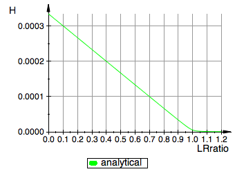
// plot analytical solution
Req_analytical:= plot::Function2d(
Function=(fReq_U_R_RL(Total_R, Total_R*LRratio, Ka1, Kb1, Kb2)),
LegendText="analytical",
Color = RGB::Green,
XMin=(0),
XMax=(LRratio_max),
XName=(LRratio),
TitlePositionX=(0)):
plot(Req_analytical, YAxisTitle="H",
Height=90, Width=120,TicksLabelFont=["Helvetica",12,[0,0,0],Left],
AxesTitleFont=["Helvetica",14,[0,0,0],Left],
XGridVisible=TRUE, YGridVisible=TRUE,
LegendVisible=TRUE, LegendFont=["Helvetica",14,[0,0,0],Left]);

Define all other functions
[RL]
eq_RLeq;
pnRLeq:= proc(Total_R, LRratio, Ka1, Kb1, Kb2)
// Parameter names should be different from
// variable names used in the equation!!!
local R, L;
begin
L:=pnLeq(Total_R, LRratio, Ka1, Kb1, Kb2);
R:=pnReq(Total_R, LRratio, Ka1, Kb1, Kb2);
// Equation for [RL]
eq_RLeq | Rtot=Total_R | Leq=L | Req=R | K_A_1=Ka1 | K_B_1=Kb1 | K_B_2=Kb2;
end_proc
![]()
![]()
[R*]
eq_Rstareq;
pnRstareq:= proc(Total_R, LRratio, Ka1, Kb1, Kb2)
// Parameter names should be different from
// variable names used in the equation!!!
local L, RL;
begin
L:=pnLeq(Total_R, LRratio, Ka1, Kb1, Kb2);
RL:=pnRLeq(Total_R, LRratio, Ka1, Kb1, Kb2);
// Equation for [RL]
eq_Rstareq | Rtot=Total_R | Leq=L | RLeq=RL | K_A_1=Ka1 | K_B_1=Kb1 | K_B_2=Kb2;
end_proc

![]()
[R*L]
eq_RstarLeq;
pnRstarLeq:= proc(Total_R, LRratio, Ka1, Kb1, Kb2)
// Parameter names should be different from
// variable names used in the equation!!!
local RL;
begin
RL:=pnRLeq(Total_R, LRratio, Ka1, Kb1, Kb2);
// Equation for [RL]
eq_RstarLeq | Rtot=Total_R | RLeq=RL | K_A_1=Ka1 | K_B_1=Kb1 | K_B_2=Kb2;
end_proc
![]()
![]()
Test functioning of the procedures:
pnLeq(1, 1, 1, 2, 3);
pnReq(1, 1, 1, 2, 3);
pnRLeq(1, 1, 1, 2, 3);
pnRstareq(1, 1, 1, 2, 3);
pnRstarLeq(1, 1, 1, 2, 3);
![]()
![]()
![]()
![]()
![]()
Make wrapper functions for plotting
fnRLeq:=LRratio -> pnRLeq(Total_R, LRratio, Ka1, Kb1, Kb2);
fnRstareq:=LRratio -> pnRstareq(Total_R, LRratio, Ka1, Kb1, Kb2);
fnRstarLeq:=LRratio -> pnRstarLeq(Total_R, LRratio, Ka1, Kb1, Kb2);


Create plots
Leq_numeric:= plot::Function2d(
Function=(fnLeq),
LegendText="[L]",
Color = RGB::Green,
XMin=(0),
XMax=(LRratio_max),
XName=(LRratio),
TitlePositionX=(0)):
// plot numeric solution
Req_numeric:= plot::Function2d(
Function=(fnReq1),
LegendText="[R]",
Color = RGB::Black,
XMin=(0),
XMax=(LRratio_max),
XName=(LRratio),
TitlePositionX=(0)):
// plot numeric solution
RLeq_numeric:= plot::Function2d(
Function=(fnRLeq),
LegendText="[RL]",
Color = RGB::Blue,
XMin=(0),
XMax=(LRratio_max),
XName=(LRratio),
TitlePositionX=(0)):
// plot numeric solution
Rstareq_numeric:= plot::Function2d(
Function=(fnRstareq),
LegendText="[R*]",
Color = RGB::Red,
XMin=(0),
XMax=(LRratio_max),
XName=(LRratio),
TitlePositionX=(0)):
// plot numeric solution
RstarLeq_numeric:= plot::Function2d(
Function=(fnRstarLeq),
LegendText="[R*L]",
Color = RGB::Magenta,
XMin=(0),
XMax=(LRratio_max),
XName=(LRratio),
TitlePositionX=(0)):
plot(Leq_numeric, Req_numeric, RLeq_numeric, Rstareq_numeric, RstarLeq_numeric,
YAxisTitle="M",
Height=180, Width=160,TicksLabelFont=["Helvetica",12,[0,0,0],Left],
AxesTitleFont=["Helvetica",14,[0,0,0],Left],
XGridVisible=TRUE, YGridVisible=TRUE,
LegendVisible=TRUE, LegendFont=["Helvetica",14,[0,0,0],Left]);
Comparison of graphs obtained with analytical and numeric solutions
|
Analytical solution Total_R:=1e-3: Ka1:=1e7: Kb1:=2/1: Kb2:=0.1:
|
Numeric solution Total_R:=1e-3: Ka1:=1e7: Kb1:=2/1: Kb2:=0.1: |
|
|
|
Conclusion:
My numeric solutions are indistinguishable from analytical.
7. Save results on disk for future use
(you can retrieve them later by executing: fread(filename,Quiet))
ProjectName
![]()
Save basic equations and corresponding procedures
filename:=CurrentPath.ProjectName."_numeric_solutions.mb";
write(filename,
fRtot, pnLeq,
eq_Req, pnReq,
eq_RLeq, pnRLeq,
eq_Rstareq, pnRstareq,
eq_RstarLeq, pnRstarLeq,
KA2_U_R_RL
)
![]()
Conclusions
1. I analyzed analytical solutions for the U_R_RL system
2. Procedure for numeric solving is presented here
3. Make sure boundary conditions for Leq search don't start with 0, otherwise the solver fails!!! It means I should not use numeric results when extrapolating to LRratio=0.
4. You may load numeric solutions as described in
Equilibria/U_R_RL_load_example.mn