Testing the I_ab model
The I_ab model is the simplest two-state isomerization model
Contents
close all
clear all
Here you will find all figures
figures_folder='I_ab_testing_figures';
Test Computation of Equilibrium Concentrations
Set some meaningful parameters
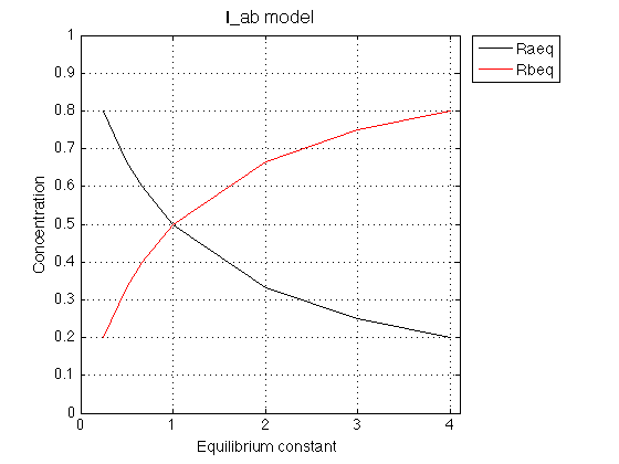
Rtotal=1; % Receptor concentration, M
K_As=[0.25 0.5 0.667 1 2 3 4];  % Binding affinity constant

% Set appropriate options for the model (see model file for details)
model_numeric_solver='analytical'  ;
model_numeric_options='n/a';

concentrations_array=[];
for counter=1:length(K_As)
    % compute
    [concentrations species_names] = equilibrium_thermodynamic_equations.I_ab_model(...
        Rtotal, K_As(counter),...
        model_numeric_solver, model_numeric_options);
    % collect
    concentrations_array = [concentrations_array ; concentrations];
end
Plot
Figure_title= 'I_ab model';
X_range=[0 max(K_As)+0.1 ]; % extend X just a bit past last point
Y_range=[0 Rtotal ]; % keep automatic scaling for Y
% display figure
figure_handle=equilibrium_thermodynamic_equations.plot_populations(...
    K_As, concentrations_array, species_names, Figure_title, X_range, Y_range);
xlabel('Equilibrium constant','FontSize',14);
% save it
results_output.output_figure(figure_handle, figures_folder, 'Concentrations_plot');
Observations
The ratio between Ra and Rb forms changes appropriately with K_A value.
Conclusion
The model equilibrium_thermodynamic_equations.I_ab_model() works well.
Test of NMR line shape calculations
We will generate line shapes for in conditions where we can expect specific patterns. We will plot a spectrum at a specific solution conditions (we will not use Series of datasets for simplicity).
Create NMR line shape dataset
Create data object for 1D NMR line shapes
test1=NMRLineShapes1D('Simulation','Test_1');
test1.set_active_model('I_ab-model', model_numeric_solver, model_numeric_options)
test1.show_active_model() % to look up necessary parameters of the model
ans =

Active model:
Model 2:  "I_ab-model"
Model description
"Two-state intramolecular isomerization, analytical"
Model handle: line_shape_equations_1D.I_ab_model_1D
Current solver: analytical
Model parameters:
1: Rtotal     2: K_A     3: k_2_A     4: w0_Ra     5: w0_Rb     6: FWHH_Ra     7: FWHH_Rb     8: ScaleFactor
Set range for X to extend beyond resonances
w_min= -300;
w_max= 500;
datapoints=100;  % Does not matter much because smooth curve is anyway calculated
test1.set_X(linspace(w_min, w_max, datapoints));
Set fixed plotting ranges for easier comparison If we do not set ranges they will be chosen automatically for each graph
test1.X_range=[w_min w_max]; % this sets display range in the plots
test1.Y_range=[0 8e-5]; % this sets display range in the plots
Calculate ideal data: set noise RMSD to 0 for both X and Y
X_RMSD=0;
Y_RMSD=0;
Test 1:
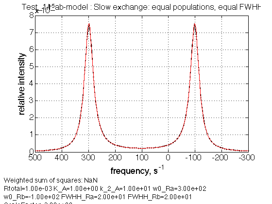
test_number=1;
name='Slow exchange: equal populations, equal FWHH'
% Use the same thermodynamic parameters as above. Add spectral and kinetic parameters:
Rtotal=1e-3;
K_A=1;          % equilibrium constant
k_2_A=10;   % reverse rate constant , 1/s
w0_Ra=300;    % NMR frequency , 1/s
w0_Rb=-100;      % NMR frequency , 1/s
FWHH_Ra=20;    % line width at half height of the peak, 1/s
FWHH_Rb=20; % line width at half height of the peak, 1/s
ScaleFactor=3;     % a multiplier for spectral amplitude (used only when fitting data)

% compute equilbrium concentrations
[concentrations species_names] = equilibrium_thermodynamic_equations.I_ab_model(...
        Rtotal, K_A,...
        model_numeric_solver, model_numeric_options);


% plot line shapes
parameters=[    Rtotal    K_A    k_2_A   w0_Ra   w0_Rb   FWHH_Ra    FWHH_Rb    ScaleFactor  ];

test1.simulate_noisy_data(parameters, X_RMSD, Y_RMSD);
figure_handle=test1.plot_simulation(name);
results_output.output_figure(figure_handle, figures_folder, sprintf('Test_results.%d', test_number));
name =

Slow exchange: equal populations, equal FWHH
Observations
We see a correct 1:1 intensity ratio, peak positioning and the line widths
Test 2
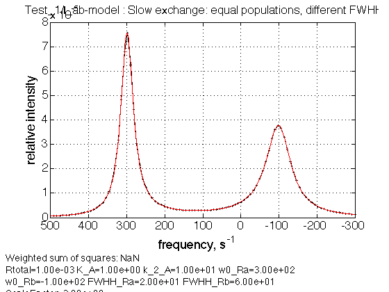
test_number=2;
name='Slow exchange: equal populations, different FWHH';
% Use the same thermodynamic parameters as above. Add spectral and kinetic parameters:
Rtotal=1e-3;
K_A=1;          % equilibrium constant
k_2_A=10;   % reverse rate constant , 1/s
w0_Ra=300;    % NMR frequency , 1/s
w0_Rb=-100;      % NMR frequency , 1/s
FWHH_Ra=20;    % line width at half height of the peak, 1/s
FWHH_Rb=60; % line width at half height of the peak, 1/s
ScaleFactor=3;     % a multiplier for spectral amplitude (used only when fitting data)

% compute equilbrium concentrations
[concentrations species_names] = equilibrium_thermodynamic_equations.I_ab_model(...
        Rtotal, K_A,...
        model_numeric_solver, model_numeric_options);


% plot line shapes
parameters=[    Rtotal    K_A    k_2_A   w0_Ra   w0_Rb   FWHH_Ra    FWHH_Rb    ScaleFactor  ];

test1.simulate_noisy_data(parameters, X_RMSD, Y_RMSD);
figure_handle=test1.plot_simulation(name);
results_output.output_figure(figure_handle, figures_folder, sprintf('Test_results.%d', test_number));
Observations
We see an expected broadening of Rb.
Test 3
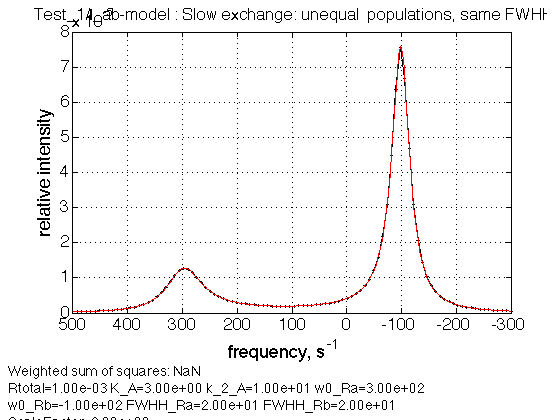
test_number=3;
name='Slow exchange: unequal  populations, same FWHH';
% Use the same thermodynamic parameters as above. Add spectral and kinetic parameters:
Rtotal=1e-3;
K_A=3;          % equilibrium constant
k_2_A=10;   % reverse rate constant , 1/s
w0_Ra=300;    % NMR frequency , 1/s
w0_Rb=-100;      % NMR frequency , 1/s
FWHH_Ra=20;    % line width at half height of the peak, 1/s
FWHH_Rb=20; % line width at half height of the peak, 1/s
ScaleFactor=2;     % a multiplier for spectral amplitude (used only when fitting data)

% compute equilbrium concentrations
[concentrations species_names] = equilibrium_thermodynamic_equations.I_ab_model(...
        Rtotal, K_A,...
        model_numeric_solver, model_numeric_options);


% plot line shapes
parameters=[    Rtotal    K_A    k_2_A   w0_Ra   w0_Rb   FWHH_Ra    FWHH_Rb    ScaleFactor  ];

test1.simulate_noisy_data(parameters, X_RMSD, Y_RMSD);
figure_handle=test1.plot_simulation(name);
results_output.output_figure(figure_handle, figures_folder, sprintf('Test_results.%d', test_number));
Observations
We see an expected preferential broadening of Ra. Therefore, intensity ratio is > K_A
Test 4
test_number=4;
name='Fast exchange: unequal  populations, same FWHH';
% Use the same thermodynamic parameters as above. Add spectral and kinetic parameters:
Rtotal=1e-3;
K_A=3;          % equilibrium constant
k_2_A=500;   % reverse rate constant , 1/s
w0_Ra=300;    % NMR frequency , 1/s
w0_Rb=-100;      % NMR frequency , 1/s
FWHH_Ra=20;    % line width at half height of the peak, 1/s
FWHH_Rb=20; % line width at half height of the peak, 1/s
ScaleFactor=2;     % a multiplier for spectral amplitude (used only when fitting data)

% compute equilbrium concentrations
[concentrations species_names] = equilibrium_thermodynamic_equations.I_ab_model(...
        Rtotal, K_A,...
        model_numeric_solver, model_numeric_options);


% plot line shapes
parameters=[    Rtotal    K_A    k_2_A   w0_Ra   w0_Rb   FWHH_Ra    FWHH_Rb    ScaleFactor  ];

test1.simulate_noisy_data(parameters, X_RMSD, Y_RMSD);
figure_handle=test1.plot_simulation(name);
results_output.output_figure(figure_handle, figures_folder, sprintf('Test_results.%d', test_number));
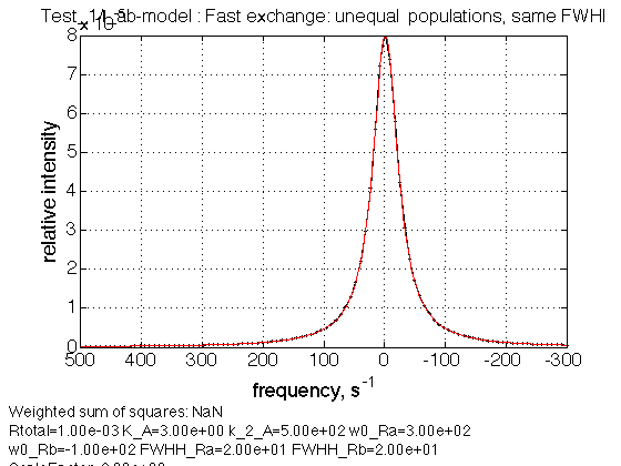
Observations
We see an expected averaged peak at 3:1 position between the frequencies of species
Conclusions
The I_ab model works as expected.