U-R_RL
Derivation of differential equations describing evolution of spin concentrations
1. Reaction rates and partial conversion rates
4. Expression in terms of spin (monomer) concentrations
clean up workspace
reset()
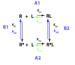
Write properly balanced reactions equations:
Write properly balanced reactions equations:
Transition A1:
(1) (2)
R+L<=>RL
Constants: k_1_A1 (forward), k_2_A1 (reverse).
Transition A2:
(1) (2)
R*+L<=>RL*
Constants: k_1_A2 (forward), k_2_A2 (reverse).
Transition B1:
(1) (2)
R <=> R*
Constants: k_1_B1 (forward), k_2_B1 (reverse).
Transition B2:
(1) (2)
RL <=> RL*
Constants: k_1_B2 (forward), k_2_B2 (reverse).
Write reaction rates
We distinguish reaction rates ( Rate, elementary reaction acts per unit time) and conversion rates (dc/dt, number of moles of specific species consumed/produced per unit time). Conversion rates, dc/dt, for species are related to reaction rates, Rate, through molecularity coefficients.
We also distinguish here partial conversion rates from net (overall) conversion rates. The net conversion rate is actual rate of change in measured concentration of the species. Partial conversion rate is the conversion rate of the species along a specific branch of the reaction mechanism. Summing partial conversion rates of the species one obtains the net conversion rate.
NOTE: In this mechanism all transition involve only one molecules of species of each kind, therefore all partial conversion rates are equal to reaction rates.
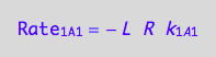
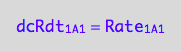
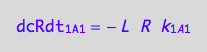
Ligand binding to R (forward transition on A1: 1_A1)
a reaction rate
eq1_1a:= Rate_1_A_1 = -k_1_A_1*R*L
a partial conversion rate of R
eq1_1b:= dcRdt_1_A_1 = Rate_1_A_1
The final form
eq1_1c:= eq1_1b | eq1_1a

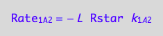
Ligand binding to R* (forward transition on A2: 1_A2)
a reaction rate
eq1_2a:= Rate_1_A_2 = - k_1_A_2*Rstar*L
a partial conversion rate of Rstar
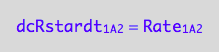
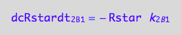
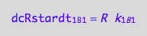
eq1_2b:= dcRstardt_1_A_2 = Rate_1_A_2
The final form
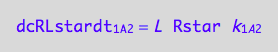
eq1_2c:= eq1_2b | eq1_2a

RL dissociation (reverse transition on A1: 2_A1)
a reaction rate
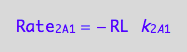
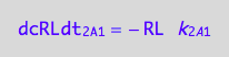
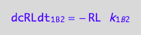
eq1_3a:= Rate_2_A_1 = -k_2_A_1 * RL
a partial conversion rate
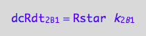
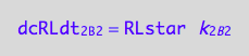
eq1_3b:= dcRLdt_2_A_1 = Rate_2_A_1

The final form
eq1_3c:= eq1_3b |eq1_3a

RL* dissociation rate (reverse transition on A2: 2_A2)
a reaction rate
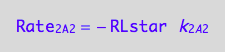
eq1_4a:= Rate_2_A_2 = - k_2_A_2 * RLstar
a partial conversion rate
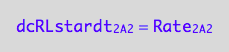
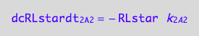
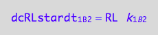
eq1_4b:= dcRLstardt_2_A_2 = Rate_2_A_2
Final form
eq1_4c:= eq1_4b | eq1_4a
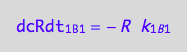
R isomerization (forward transition on B1: 1_B1)
a reaction rate
eq1_5a:= Rate_1_B_1 = - k_1_B_1 * R
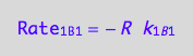
a partial conversion rate
eq1_5b:= dcRdt_1_B_1 = Rate_1_B_1

The final form
eq1_5c:= eq1_5b | eq1_5a

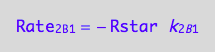
R* isomerization (reverse transition on B1: 1_B1)
a reaction rate
eq1_6a:= Rate_2_B_1 = -k_2_B_1 * Rstar
a partial conversion rate
eq1_6b:= dcRstardt_2_B_1 = Rate_2_B_1

The final form
eq1_6c:= eq1_6b | eq1_6a

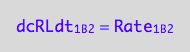
RL isomerization (forward transition on B2: 1_B2)
a reaction rate
eq1_7a:= Rate_1_B_2 = -k_1_B_2 * RL

a partial conversion rate
eq1_7b:= dcRLdt_1_B_2 = Rate_1_B_2
The final form
eq1_7c:= eq1_7b | eq1_7a

RL* isomerization (reverse transition on B2: 2_B2)
a reaction rate
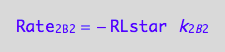
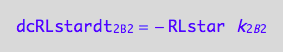
eq1_8a:= Rate_2_B_2 = -k_2_B_2 *RLstar
a partial conversion rate
eq1_8b:= dcRLstardt_2_B_2 = Rate_2_B_2

The final form
eq1_8c:= eq1_8b | eq1_8a
To define evolution of the species we need to compute concentrations as a function of time. To this end, we will write differential equations for conversion rates of all species.
In a reversible process both forward and reverse reaction occur simultaneously. Thus, the net conversion rate of the species is a difference between partial conversion rates resulting from forward and reverse reactions, summed along all branches.
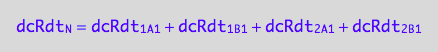
Net conversion rate of R
Sum all pertaining partial rates with respective signs
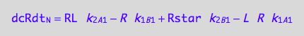
eq3_1a:= dcRdt_N = dcRdt_1_A_1 + dcRdt_2_A_1 + dcRdt_1_B_1 + dcRdt_2_B_1
What are the terms?
Negative terms
eq1_1c
eq1_5c
Positive terms (use mass conservation principle)
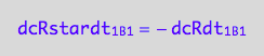
dcRdt_2_A_1 = -dcRLdt_2_A_1;
eq3_1b:= % | eq1_3c
dcRdt_2_B_1 = -dcRstardt_2_B_1;
eq3_1c:= % | eq1_6c
Assemble the net conversion rate
eq3_1d:= eq3_1a | eq1_1c | eq1_5c | eq3_1b | eq3_1c
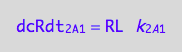
Net conversion rate of RL
Sum all pertaining partial rates with respective signs
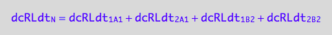
eq3_2a:= dcRLdt_N = dcRLdt_1_A_1 + dcRLdt_2_A_1 + dcRLdt_1_B_2 + dcRLdt_2_B_2
What are the terms?
Negative terms
eq1_3c
eq1_7c
Positive terms (use mass conservation principle)
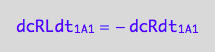
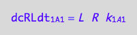
dcRLdt_1_A_1 = -dcRdt_1_A_1;
eq3_2b:= % | eq1_1c
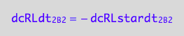
dcRLdt_2_B_2 = -dcRLstardt_2_B_2;
eq3_2c:= % | eq1_8c
Assemble the equation for a net rate
eq3_2d:= eq3_2a | eq1_3c | eq1_7c | eq3_2b | eq3_2c

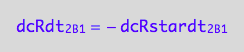
Net conversion rate of R*
Sum all pertaining partial rates with respective signs
eq3_3a:= dcRstardt_N = dcRstardt_1_B_1 + dcRstardt_2_B_1 + dcRstardt_1_A_2 + dcRstardt_2_A_2

what are the terms?
Negative terms
eq1_6c
eq1_2c
Positive terms (use mass conservation principle)
dcRstardt_1_B_1 = -dcRdt_1_B_1;
eq3_3b:= % | eq1_5c
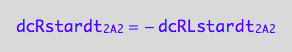
dcRstardt_2_A_2 = - dcRLstardt_2_A_2;
eq3_3c:= % | eq1_4c
Assemble equation for the net rate
eq3_3d:= eq3_3a | eq1_6c | eq1_2c | eq3_3b | eq3_3c

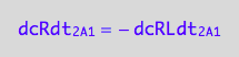
Net conversion rate of RL*
Sum all pertaining partial rates with respective signs
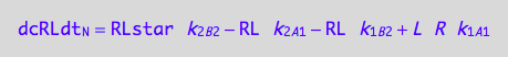
eq3_4a:= dcRLstardt_N = dcRLstardt_1_B_2 + dcRLstardt_2_B_2 + dcRLstardt_1_A_2 + dcRLstardt_2_A_2

what are the terms?
Negative terms
eq1_8c

eq1_4c

Positive terms (use mass conservation principle)
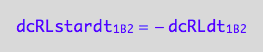
dcRLstardt_1_B_2 = - dcRLdt_1_B_2;
eq3_4b:= % | eq1_7c
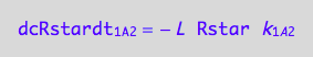
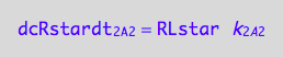
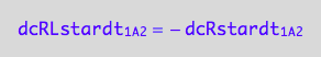
dcRLstardt_1_A_2 = - dcRstardt_1_A_2;
eq3_4c:= % | eq1_2c
Assemble equation for the net rate
eq3_4d:= eq3_4a | eq1_8c | eq1_4c | eq3_4b | eq3_4c

not needed here because we do not have oligomerization reactions.
Summarize the derivation results
eq3_1d

eq3_3d

eq3_2d
eq3_4d

Assign order to species
eq5_1a:= R = C1;
eq5_1b:= Rstar= C2;
eq5_1c:= RL = C3;
eq5_1d:= RLstar=C4;


Same order for net rates
eq5_2a:= dcRdt_N = dC1dt;
eq5_2b:= dcRstardt_N = dC2dt;
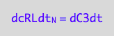
eq5_2c:= dcRLdt_N = dC3dt;
eq5_2d:= dcRLstardt_N = dC4dt;

Restate the equations (rename free ligand concentration too)
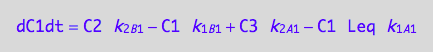
eq5_3a:= eq3_1d | eq5_1a | eq5_1b | eq5_1c | eq5_1d | eq5_2a | eq5_2b | eq5_2c | eq5_2d | L = Leq
eq5_3b:= eq3_3d | eq5_1a | eq5_1b | eq5_1c | eq5_1d | eq5_2a | eq5_2b | eq5_2c | eq5_2d | L = Leq
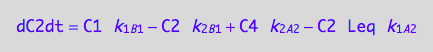
eq5_3c:= eq3_2d | eq5_1a | eq5_1b | eq5_1c | eq5_1d | eq5_2a | eq5_2b | eq5_2c | eq5_2d | L = Leq
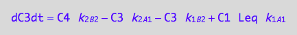
eq5_3d:= eq3_4d | eq5_1a | eq5_1b | eq5_1c | eq5_1d | eq5_2a | eq5_2b | eq5_2c | eq5_2d | L = Leq
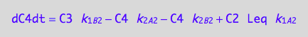
Prepare results for transfer to MATLAB
To avoid typing errors when transfering derived K matrix to MATLAB we type it in here and then directly test against derivation result. Then K matrix may be transfered to MATLAB by cut-and-paste of the MuPad output.
Enter the K-matrix looking at the above results (collect terms at correspondingly numbered species).
Simple rules that allow catching mistakes in K matrix derivation:
(1) a sum of each column should be zero (so each constant must appear with both positive and negative sign), and
(2) each row has to have complete pairs of constants (i.e., if k12
appears there must be k21 in the same row with an opposite sign and so on).
K:=matrix(4,4,[
[ -k_1_B_1-k_1_A_1*Leq, k_2_B_1, k_2_A_1, 0 ],
[ k_1_B_1, -k_2_B_1 -k_1_A_2*Leq, 0, k_2_A_2 ],
[ k_1_A_1*Leq, 0 , -k_2_A_1 -k_1_B_2, k_2_B_2 ],
[ 0 , k_1_A_2*Leq, k_1_B_2, -k_2_A_2 - k_2_B_2 ]
])
![matrix([[- k_1_B_1 - Leq*k_1_A_1, k_2_B_1, k_2_A_1, 0], [k_1_B_1, - k_2_B_1 - Leq*k_1_A_2, 0, k_2_A_2], [Leq*k_1_A_1, 0, - k_1_B_2 - k_2_A_1, k_2_B_2], [0, Leq*k_1_A_2, k_1_B_2, - k_2_A_2 - k_2_B_2]])](U_R_RL_images/math72.png)
Create a column vector of species concentrations
P:=matrix(4,1,[C1, C2, C3, C4])
![matrix([[C1], [C2], [C3], [C4]])](U_R_RL_images/math73.png)
Check correctness of the entered K matrix by multiplying with P and comparing to the above equations:
Multiply K and P:
dCdt_manual_input:= K*P
![matrix([[C2*k_2_B_1 + C3*k_2_A_1 - C1*(k_1_B_1 + Leq*k_1_A_1)], [C1*k_1_B_1 + C4*k_2_A_2 - C2*(k_2_B_1 + Leq*k_1_A_2)], [C4*k_2_B_2 - C3*(k_1_B_2 + k_2_A_1) + C1*Leq*k_1_A_1], [C3*k_1_B_2 - C4*(k_2_A_2 + k_2_B_2) + C2*Leq*k_1_A_2]])](U_R_RL_images/math74.png)
Collect right-hand-side parts of equations
dCdt_mupad:=matrix(4,1,[ rhs(eq5_3a), rhs(eq5_3b), rhs(eq5_3c), rhs(eq5_3d)])
![matrix([[C2*k_2_B_1 - C1*k_1_B_1 + C3*k_2_A_1 - C1*Leq*k_1_A_1], [C1*k_1_B_1 - C2*k_2_B_1 + C4*k_2_A_2 - C2*Leq*k_1_A_2], [C4*k_2_B_2 - C3*k_2_A_1 - C3*k_1_B_2 + C1*Leq*k_1_A_1], [C3*k_1_B_2 - C4*k_2_A_2 - C4*k_2_B_2 + C2*Leq*k_1_A_2]])](U_R_RL_images/math75.png)
Compare derivation result to manual input
dCdt_mupad=dCdt_manual_input:
normal(%);
bool(%)
![matrix([[C2*k_2_B_1 - C1*k_1_B_1 + C3*k_2_A_1 - C1*Leq*k_1_A_1], [C1*k_1_B_1 - C2*k_2_B_1 + C4*k_2_A_2 - C2*Leq*k_1_A_2], [C4*k_2_B_2 - C3*k_2_A_1 - C3*k_1_B_2 + C1*Leq*k_1_A_1], [C3*k_1_B_2 - C4*k_2_A_2 - C4*k_2_B_2 + C2*Leq*k_1_A_2]]) = matrix([[C2*k_2_B_1 - C1*k_1_B_1 + C3*k_2_A_1 - C1*Leq*k_1_A_1], [C1*k_1_B_1 - C2*k_2_B_1 + C4*k_2_A_2 - C2*Leq*k_1_A_2], [C4*k_2_B_2 - C3*k_2_A_1 - C3*k_1_B_2 + C1*Leq*k_1_A_1], [C3*k_1_B_2 - C4*k_2_A_2 - C4*k_2_B_2 + C2*Leq*k_1_A_2]])](U_R_RL_images/math76.png)

=> Typed K-matrix is correct.
Use this K-matrix (copy-paste output to MATLAB)
K;
![matrix([[- k_1_B_1 - Leq*k_1_A_1, k_2_B_1, k_2_A_1, 0], [k_1_B_1, - k_2_B_1 - Leq*k_1_A_2, 0, k_2_A_2], [Leq*k_1_A_1, 0, - k_1_B_2 - k_2_A_1, k_2_B_2], [0, Leq*k_1_A_2, k_1_B_2, - k_2_A_2 - k_2_B_2]])](U_R_RL_images/math78.png)
Differential equations governing spin populations in U-R-RL system have been derived. The K matrix has been prepared for transferring to MATLAB.