U_R2_FWHHconstr

Tutorial 8. Testing a U_R2_FWHHconstr
TEST COMPUTATION OF EQUILIBRIUM POPULATIONS
TEST OF NMR LINE SHAPE CALCULATION FOR U_R2_FWHHconstr
Create NMR line shape dataset
1. Slow exchange in free receptor
2. Introduce increased line width of the dimer
3. Introduce EM line broadening
4. Dilution of free receptor
5. Fast exchange in free receptor
6. Concentrated: Return to the original condition
7. A fully saturated receptor
8. Same as previous but with assuming correction to ligand concentration
Create a titration series
CONCLUSIONS

Tutorial 8. Testing a U_R2_FWHHconstr

this is a model with dimerization of the free receptor with a pre-set relationship between the line widths of the monomer and a dimer

close all
clear all

Here you will find all figures

figures_folder='testing_figures';
% *Prepare TotalFit session for easy display of many graphs*
storage_session=TotalFit('All_tests');

TEST COMPUTATION OF EQUILIBRIUM POPULATIONS

Set some meaningful parameters

Rtotal=1e-3; % Receptor concentration, M
LRratio_array=[1e-3 0.1 0.2 0.3 0.4 0.5 0.6 0.7 0.8 0.9 1.0 1.1 1.2]; % Array of L/R
K_a_A=1e6;  % Binding affinity constant
K_a_B=5e3 ;  % Dimerization constant

% Set appropriate options for the model (see model file for details)
model_numeric_solver='fminbnd'  ;

model_numeric_options=optimset('Diagnostics','off', ...
                    'Display','off',...
                    'TolX',1e-9,...
                    'MaxFunEvals', 1e9);

Important option here is TolX that sets termination tolerance on free ligand concentation in molar units. With our solution concentrations in 1e-3 range TolX should be set to some 1e-9.

Compute arrays for populations and plot

concentrations_array=[];
for counter=1:length(LRratio_array)
    % compute
    [concentrations species_names] = equilibrium_thermodynamic_equations.U_R2_model(...
        Rtotal, LRratio_array(counter), K_a_A, K_a_B,...
        model_numeric_solver, model_numeric_options);
    % collect
    concentrations_array = [concentrations_array ; concentrations];
end

Plot

Figure_title= 'U-R2 populations';
X_range=[0 max(LRratio_array)+0.1 ]; % extend X just a bit past last point
Y_range=[ ]; % keep automatic scaling for Y
% display figure
figure_handle=equilibrium_thermodynamic_equations.plot_populations(...
    Rtotal*ones(length(LRratio_array),1),...
    LRratio_array, concentrations_array, species_names, Figure_title, X_range, Y_range);
% save it
results_output.output_figure(figure_handle, figures_folder, 'Concentrations_plot');

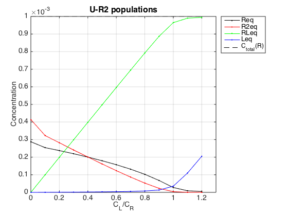
Observations The result is exactly what we expect from this model. In absence of a ligand the receptor exists in equilibrium between monomer, R, and a dimer, R2. Since one molecule of dimer is made of two monomers, the total concentration of a dimer has to be doubled to see concentration of the monomers in the dimer form. A sum of monomer concentration in free and dimer form is equal to Rtotal we set.

As ligand is added, the RL species is formed, leading to reduction of total concentration of the receptor. This reduction leads shifting of R<=>R2 equilibrium towards monomeric species such that above molar ratio L/R=0.4 the monomer becomes a major species in solution. This is the same effect as dilution of the receptor solution: progressive depletion of R2 population.

Once the receptor approaches saturation, the RL concentration approaches the Rtotal set above. At the same time, the free ligand begins to accumulate linearly with L/R molar ratio.

Conclusion

The model equilibrium_thermodynamic_equations.U_R2_model() works well.

TEST OF NMR LINE SHAPE CALCULATION FOR U_R2_FWHHconstr

We will generate line shapes for U-R2 in conditions where we can expect specific patterns. We will plot a spectrum at a specific solution conditions (we will not use Series of datasets for simplicity).

1. Ligand-free receptor in slow exchange should show two separate peaks with areas proportional to their equilibrium concentrations. This ratio should change upon dilution in favor of the monomer. NOTE: NMR intensity is proportional to concentrations of NMR-active spins so it will track concentration of monomers in monomeric and dimeric structures.

2. Setting the line width parameter should respectively show in the line shapes

3. Fast exchange in the same setting should reveal population-weighted average peak. Here, again, the concentration of monomers in free and dimeric form will be important---not the concentration of dimeric species. Similarly, dilution would lead to a shift of a peak towards frequency of monomeric species.

4. Addition of saturating concentration of ligand should give us a single peak at the RL frequency.

Create NMR line shape dataset

Create data object for 1D NMR line shapes

test1=NMRLineShapes1D('Simulation','Test_1');
test1.set_active_model('U_R2_FWHHconstr-model', model_numeric_solver, model_numeric_options)
test1.show_active_model() % to look up necessary parameters of the model

ans =
Active model:
Model 11:  "U_R2_FWHHconstr-model"
Model description
"1D NMR line shape for the U-R2 model with constrained FWHH for R and R2, no temperature/field dependence, fminbnd solver"
Model handle: line_shape_equations_1D.U_R2_FWHHconstr_model_1D
Current solver: fminbnd
Model parameters: 
1: Rtotal     2: LRratio     3: log10(K_A)     4: log10(K_B)     5: k_2_A     6: k_2_B     7: w0_R     8: w0_R2     9: w0_RL     10: FWHH_R_monomer     11: FWHH_R2_R_ratio     12: FWHH_RL     13: EM_line_broadening_Hz     14: ScaleFactor     15: LRcorrection

Set range for X to extend beyond resonances

w_min= -300;
w_max= 500;
datapoints=100;  % Does not matter much because smooth curve is anyway calculated
test1.set_X(linspace(w_min, w_max, datapoints));

Set fixed plotting ranges for easier comparison If we do not set ranges they will be chosen automatically for each graph

test1.X_range=[w_min w_max]; % this sets display range in the plots
test1.Y_range=[0 8e-5]; % this sets display range in the plots

Calculate ideal data: set noise RMSD to 0 for both X and Y

X_RMSD=0;
Y_RMSD=0;

1. Slow exchange in free receptor

test1.set_name('1. Slow exchange in free receptor');
% Use the same thermodynamic parameters as above. Add spectral and kinetic parameters:
LRratio = 0.01 ;  % NOTE: for numeric model this value has to be >=0.01
Log10_K_A = log10(K_a_A);
Log10_K_B = log10(K_a_B);
k_2_A    = 1;   % dissociation rate constant of the complex, 1/s
k_2_B    = 1;   % dissociation rate constant of the receptor dimer, 1/s
w0_R     = -200;    % NMR frequency of the free receptor R, 1/s
w0_R2    = 200;  % NMR frequency of the dimer R2, 1/s
w0_RL    = 400;  % NMR frequency of the bound complex RL, 1/s
FWHH_R_monomer   = 20;     % line width at half height of the peak of R, 1/s
FWHH_R2_R_ratio  = 1;     % factor to multiply natural line width of R with to obtain natural line width of R2
FWHH_RL  = 20;     % line width at half height of the peak of RL, 1/s
EM_line_broadening_Hz = 0; % line broadening contribution from EM apodization window present in FWHH, Hz
ScaleFactor = 1;  % a multiplier for spectral amplitude (used only when fitting data)
LRcorrection = 1; % multiplier for L/R ratio values.

% compute equilbrium concentrations
[concentrations species_names] = equilibrium_thermodynamic_equations.U_R2_model(...
        Rtotal, LRratio, K_a_A, K_a_B,...
        model_numeric_solver, model_numeric_options)


% plot line shapes
parameters=[ Rtotal  LRratio   Log10_K_A   Log10_K_B  k_2_A  k_2_B ...
     w0_R  w0_R2  w0_RL ...
     FWHH_R_monomer  FWHH_R2_R_ratio  FWHH_RL  EM_line_broadening_Hz...
     ScaleFactor  LRcorrection ];


test1.simulate_noisy_data(parameters, X_RMSD, Y_RMSD);
figure_handle=test1.plot_simulation('Slow: free R');
results_output.output_figure(figure_handle, figures_folder, 'Slow_concentrated_R');
storage_session.copy_dataset_into_array(test1);

concentrations =
   1.0e-03 *
    0.2683    0.3601    0.0100    0.0000
species_names = 
    'Req'    'R2eq'    'RLeq'    'Leq'

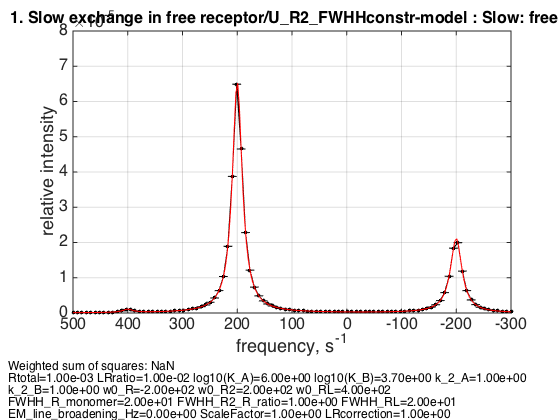
Expected ratio of R2 peak to R peak is 4:1 corresponding to number of spins experiencing dimeric and monomeric environment. Since line widths are the same the intensity is proportional to the ratio

2. Introduce increased line width of the dimer

test1.set_name('2.  Introduce increased line width of the dimer');

FWHH_R2_R_ratio  = 2;     % factor to multiply natural line width of R with to obtain natural line width of R2
% plot line shapes
parameters=[ Rtotal  LRratio   Log10_K_A   Log10_K_B  k_2_A  k_2_B ...
     w0_R  w0_R2  w0_RL ...
     FWHH_R_monomer  FWHH_R2_R_ratio  FWHH_RL  EM_line_broadening_Hz...
     ScaleFactor  LRcorrection ];


test1.simulate_noisy_data(parameters, X_RMSD, Y_RMSD);
% figure_handle=test1.plot_simulation('Dimer linewidth doubled');
% results_output.output_figure(figure_handle, figures_folder, 'Slow_concentrated_R_FWHH_R2_doubled');
storage_session.copy_dataset_into_array(test1);

% show as series
storage_session.define_series('FWHH_R2_R_ratio tests',[1 2]);
figure_handle=storage_session.plot_1D_series('FWHH_R2_R_ratio tests', 'FWHH_R2_R_ratio tests', 0);

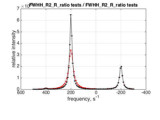
Observation: As expected the line width of the dimer doubled. Intensities are no longer 1:3 but areas should be.

3. Introduce EM line broadening

test1.set_name('3. Introduce EM line broadening');

% Have 99% of the observed FWHH be due to EM:
EM_line_broadening_Hz=(FWHH_R_monomer*0.90)/6.28; % convert to Hz
FWHH_R2_R_ratio  = 2;     % factor to multiply natural line width of R with to obtain natural line width of R2
% plot line shapes
parameters=[ Rtotal  LRratio   Log10_K_A   Log10_K_B  k_2_A  k_2_B ...
     w0_R  w0_R2  w0_RL ...
     FWHH_R_monomer  FWHH_R2_R_ratio  FWHH_RL  EM_line_broadening_Hz...
     ScaleFactor  LRcorrection ];


test1.simulate_noisy_data(parameters, X_RMSD, Y_RMSD);
% figure_handle=test1.plot_simulation('EM - 99% FWHH');
% results_output.output_figure(figure_handle, figures_folder, 'Slow_concentrated_R_EM_99prc_FWHH');
storage_session.copy_dataset_into_array(test1);

% show as series
storage_session.define_series('EM test',[1 3]);
figure_handle=storage_session.plot_1D_series('EM test', 'EM test', 0);

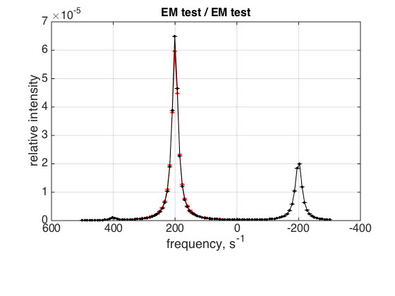
Observation: As expected, the natural line width became small because most of the observed FWHH are now due to EM line broadening effect. In this situation, doubling of the linewidth of R2 is barely observable.

4. Dilution of free receptor

test1.set_name('4. Dilution of free receptor');

Rtotal=1e-4;
EM_line_broadening_Hz=0; % remove EM broadening for clarity

% compute equilbrium concentrations
[concentrations species_names] = equilibrium_thermodynamic_equations.U_R2_model(...
        Rtotal, LRratio, K_a_A, K_a_B,...
        model_numeric_solver, model_numeric_options)



parameters=[ Rtotal  LRratio   Log10_K_A   Log10_K_B  k_2_A  k_2_B ...
     w0_R  w0_R2  w0_RL ...
     FWHH_R_monomer  FWHH_R2_R_ratio  FWHH_RL  EM_line_broadening_Hz...
     ScaleFactor  LRcorrection ];


test1.simulate_noisy_data(parameters, X_RMSD, Y_RMSD);
% figure_handle=test1.plot_simulation('Slow: 1/10 total R');
% results_output.output_figure(figure_handle, figures_folder, 'Slow_diluted_R');
% set aside for plotting later
storage_session.copy_dataset_into_array(test1);

storage_session.define_series('Dilution test',[2 4]);
figure_handle=storage_session.plot_1D_series('Dilution test', 'Dilution', 0);

concentrations =
   1.0e-04 *
    0.6140    0.1885    0.0098    0.0002
species_names = 
    'Req'    'R2eq'    'RLeq'    'Leq'

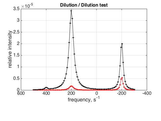
When receptor is diluted we see relative reduction in population of R2 with respect to R: peak areas are almost equal now reflecting similar number of spins in each environment (total concentration of spins, obviously, dropped due to dilution).

5. Fast exchange in free receptor

Diluted

k_2_B=1000;
parameters=[ Rtotal  LRratio   Log10_K_A   Log10_K_B  k_2_A  k_2_B ...
     w0_R  w0_R2  w0_RL ...
     FWHH_R_monomer  FWHH_R2_R_ratio  FWHH_RL  EM_line_broadening_Hz...
     ScaleFactor  LRcorrection ];


test1.simulate_noisy_data(parameters, X_RMSD, Y_RMSD);
% figure_handle=test1.plot_simulation('Fast: 1/10 R');
% results_output.output_figure(figure_handle, figures_folder, 'Fast_diluted_R');
% set aside for plotting later
storage_session.copy_dataset_into_array(test1);
storage_session.define_series('Fast exchange diluted',[ 4 5]);
figure_handle=storage_session.plot_1D_series('Fast exchange diluted', 'Diluted fast and slow', 0);

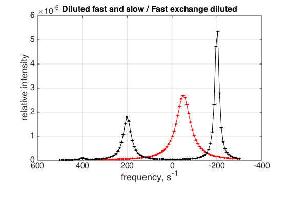
The weighted average peak has slight shift towards the monomer, because it has very slightly more spins than dimer in these conditions

6. Concentrated: Return to the original condition

Rtotal=1e-3;

% compute equilbrium concentrations
[concentrations species_names] = equilibrium_thermodynamic_equations.U_R2_model(...
        Rtotal, LRratio, K_a_A, K_a_B,...
        model_numeric_solver, model_numeric_options)



parameters=[ Rtotal  LRratio   Log10_K_A   Log10_K_B  k_2_A  k_2_B ...
     w0_R  w0_R2  w0_RL ...
     FWHH_R_monomer  FWHH_R2_R_ratio  FWHH_RL  EM_line_broadening_Hz...
     ScaleFactor  LRcorrection ];


test1.simulate_noisy_data(parameters, X_RMSD, Y_RMSD);
% figure_handle=test1.plot_simulation('Fast: 1/1 R');
% results_output.output_figure(figure_handle, figures_folder, 'Fast_concentrated_R');
% set aside for plotting later
storage_session.copy_dataset_into_array(test1);
storage_session.define_series('Fast exchange different concentrations',[ 5 6]);
figure_handle=storage_session.plot_1D_series('Fast exchange different concentrations', 'Fast - 1/10 and 1/1', 0);

concentrations =
   1.0e-03 *
    0.2683    0.3601    0.0100    0.0000
species_names = 
    'Req'    'R2eq'    'RLeq'    'Leq'

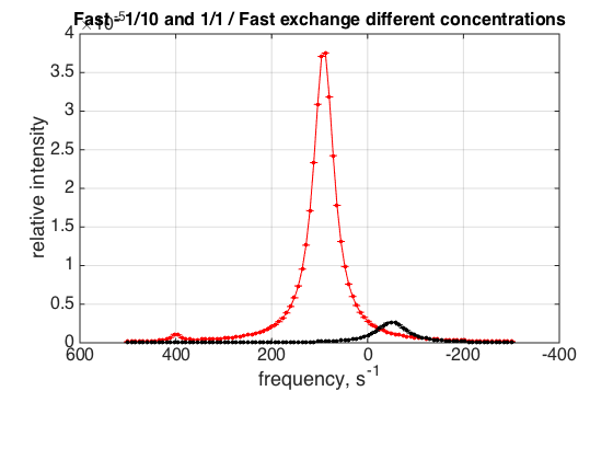
Observation: Upon concentrating the peak shifts towards the dimer: roughly at 4:1 weighted position in favor of a dimer

7. A fully saturated receptor

LRratio = 10 ;
parameters=[ Rtotal  LRratio   Log10_K_A   Log10_K_B  k_2_A  k_2_B ...
     w0_R  w0_R2  w0_RL ...
     FWHH_R_monomer  FWHH_R2_R_ratio  FWHH_RL  EM_line_broadening_Hz...
     ScaleFactor  LRcorrection ];

test1.simulate_noisy_data(parameters, X_RMSD, Y_RMSD);
% figure_handle=test1.plot_simulation('saturated RL');
% results_output.output_figure(figure_handle, figures_folder, 'Saturated_RL');
% set aside for plotting later
storage_session.copy_dataset_into_array(test1);
storage_session.define_series('Saturated RL',[ 6 7]);
figure_handle=storage_session.plot_1D_series('Saturated RL', 'R and RL', 0);

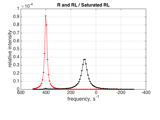
We observe a peak at a frequency of bound form

8. Same as previous but with assuming correction to ligand concentration

LRcorrection = 0.01;
parameters=[ Rtotal  LRratio   Log10_K_A   Log10_K_B  k_2_A  k_2_B ...
     w0_R  w0_R2  w0_RL ...
     FWHH_R_monomer  FWHH_R2_R_ratio  FWHH_RL  EM_line_broadening_Hz...
     ScaleFactor  LRcorrection ];

test1.simulate_noisy_data(parameters, X_RMSD, Y_RMSD);
% figure_handle=test1.plot_simulation('LRcorr=0.5');
% results_output.output_figure(figure_handle, figures_folder, 'LRcorr_0_5');
% set aside for plotting later
storage_session.copy_dataset_into_array(test1);
storage_session.define_series('LRcorrection test',[ 7 8]);
figure_handle=storage_session.plot_1D_series('LRcorrection test', 'LRcorrection  1 and 0.1', 0);

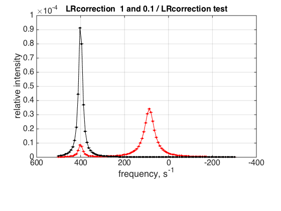
Observation The equilibrium shows a lot of unbound R/R2, as we supplied 10x less ligand versus the value of LRratio (signified by the value of LRcorrection).

Create a titration series

(see Tutorial 3 for details) Choose parameters (same as in LineShapeKin Simulation run - to compare)

Rtotal = 1e-3;
ZERO_LRratio= 0.01; % This number cannot be too small---the model is numeric and will NOT converge!
LRratio_vector=[ZERO_LRratio   0.2 0.4 0.6 0.8 1 1.5 2 3  ];
Log10_K_A = log10(1e4);
Log10_K_B = log10(1e3);
k_2_A    = 5;   % dissociation rate constant of the complex, 1/s
k_2_B    = 2000;   % dissociation rate constant of the receptor dimer, 1/s
w0_R     = 400;    % NMR frequency of the free receptor R, 1/s
w0_R2    = -400;  % NMR frequency of the dimer R2, 1/s
w0_RL    = 700;  % NMR frequency of the bound complex RL, 1/s
FWHH_R_monomer   = 90*2;     % line width at half height of the peak of R, 1/s
FWHH_R2_R_ratio  = 2;     % factor to multiply natural line width of R with to obtain natural line width of R2
FWHH_RL  = 90*2;     % line width at half height of the peak of RL, 1/s
EM_line_broadening_Hz = 0; % line broadening contribution from EM apodization window present in FWHH, Hz
ScaleFactor = 1;  % a multiplier for spectral amplitude (used only when fitting data)
LRcorrection = 1; % multiplier for L/R ratio values.

% set plotting ranges
X_range=[-500 1300];  % use old
Y_range=[];  % automatic

% choose the same parameters as above
session_name='Simulated Series';
session=TotalFit(session_name);
series_name='U_R2_FWHHconstr_simulation';
dataset_class_name='NMRLineShapes1D';
model_name='U_R2_FWHHconstr-model';
number_of_datasets=length(LRratio_vector);
X_column=linspace(X_range(1), X_range(2), 100); % use the same range

% create TotalFit session
session.create_simulation_series(series_name, dataset_class_name, model_name, ...
                 model_numeric_solver, model_numeric_options,...
                 number_of_datasets, X_column);

session.initialize_relation_matrix(sprintf('%s.all_datasets.txt', session_name));

% link parameters
parameter_number_array=[ 1    3 4 5 6 7 8 9 10 11 12 13 14 15];
session.batch_link_parameters_in_series(series_name, parameter_number_array);
session.generate_fitting_environment(sprintf('%s.fitting_environment.txt', session_name))

% prepare parameters
first_dataset_index=session.dataset_index(series_name,1);
FAKE_VALUE=1E-6;  % individual (unlinked) parameters: to be assigned later

ideal_parameters=[ Rtotal  FAKE_VALUE   Log10_K_A   Log10_K_B  k_2_A  k_2_B ...
     w0_R  w0_R2  w0_RL  FWHH_R_monomer  FWHH_R2_R_ratio  FWHH_RL EM_line_broadening_Hz...
     ScaleFactor  LRcorrection];

% prepare formal limits
fake_limits=zeros(1,length(ideal_parameters));
Monte_Carlo_range_min=fake_limits;
Monte_Carlo_range_max=fake_limits;
parameter_limits_min=fake_limits;
parameter_limits_max=fake_limits;

% assign
session.assign_parameter_values(first_dataset_index, ideal_parameters, ...
        Monte_Carlo_range_min, Monte_Carlo_range_max, parameter_limits_min, parameter_limits_max);

% Assign unlinked LRratio and ranges
parameter_number=2;
values_array=LRratio_vector;

unlinked_fake_ranges=zeros(1,number_of_datasets);
MonteCarlo_range_min_array=unlinked_fake_ranges;
MonteCarlo_range_max_array=unlinked_fake_ranges;
parameter_limits_min_array=unlinked_fake_ranges;
parameter_limits_max_array=unlinked_fake_ranges;

session.assign_unlinked_parameter_in_series(...
             series_name, parameter_number, values_array, ...
             MonteCarlo_range_min_array, MonteCarlo_range_max_array, ...
             parameter_limits_min_array, parameter_limits_max_array);

% Simulate series
X_standard_dev=0;
Y_standard_dev=1e-8;  % something really small
session.simulate_series(series_name, X_standard_dev, Y_standard_dev);

% Plot
Y_offset_percent=0;  % to offset figures vertically for easier viewing
session.set_XY_ranges_series(series_name, X_range, Y_range)
figure_handle=session.plot_1D_series(series_name, session.name, Y_offset_percent);
results_output.output_figure(figure_handle, figures_folder, 'Series');

Dataset listing is written to "Simulated Series.all_datasets.txt".

Fitting environment saved in Simulated Series.fitting_environment.txt.
ans =
New parameter relations (indexed as in all_parameters vector):

[1]     1:Rtotal | 2:Rtotal | 3:Rtotal | 4:Rtotal | 5:Rtotal | 6:Rtotal | 7:Rtotal | 8:Rtotal | 9:Rtotal
[2]     1:LRratio
[3]     1:log10(K_A) | 2:log10(K_A) | 3:log10(K_A) | 4:log10(K_A) | 5:log10(K_A) | 6:log10(K_A) | 7:log10(K_A) | 8:log10(K_A) | 9:log10(K_A)
[4]     1:log10(K_B) | 2:log10(K_B) | 3:log10(K_B) | 4:log10(K_B) | 5:log10(K_B) | 6:log10(K_B) | 7:log10(K_B) | 8:log10(K_B) | 9:log10(K_B)
[5]     1:k_2_A | 2:k_2_A | 3:k_2_A | 4:k_2_A | 5:k_2_A | 6:k_2_A | 7:k_2_A | 8:k_2_A | 9:k_2_A
[6]     1:k_2_B | 2:k_2_B | 3:k_2_B | 4:k_2_B | 5:k_2_B | 6:k_2_B | 7:k_2_B | 8:k_2_B | 9:k_2_B
[7]     1:w0_R | 2:w0_R | 3:w0_R | 4:w0_R | 5:w0_R | 6:w0_R | 7:w0_R | 8:w0_R | 9:w0_R
[8]     1:w0_R2 | 2:w0_R2 | 3:w0_R2 | 4:w0_R2 | 5:w0_R2 | 6:w0_R2 | 7:w0_R2 | 8:w0_R2 | 9:w0_R2
[9]     1:w0_RL | 2:w0_RL | 3:w0_RL | 4:w0_RL | 5:w0_RL | 6:w0_RL | 7:w0_RL | 8:w0_RL | 9:w0_RL
[10]     1:FWHH_R_monomer | 2:FWHH_R_monomer | 3:FWHH_R_monomer | 4:FWHH_R_monomer | 5:FWHH_R_monomer | 6:FWHH_R_monomer | 7:FWHH_R_monomer | 8:FWHH_R_monomer | 9:FWHH_R_monomer
[11]     1:FWHH_R2_R_ratio | 2:FWHH_R2_R_ratio | 3:FWHH_R2_R_ratio | 4:FWHH_R2_R_ratio | 5:FWHH_R2_R_ratio | 6:FWHH_R2_R_ratio | 7:FWHH_R2_R_ratio | 8:FWHH_R2_R_ratio | 9:FWHH_R2_R_ratio
[12]     1:FWHH_RL | 2:FWHH_RL | 3:FWHH_RL | 4:FWHH_RL | 5:FWHH_RL | 6:FWHH_RL | 7:FWHH_RL | 8:FWHH_RL | 9:FWHH_RL
[13]     1:EM_line_broadening_Hz | 2:EM_line_broadening_Hz | 3:EM_line_broadening_Hz | 4:EM_line_broadening_Hz | 5:EM_line_broadening_Hz | 6:EM_line_broadening_Hz | 7:EM_line_broadening_Hz | 8:EM_line_broadening_Hz | 9:EM_line_broadening_Hz
[14]     1:ScaleFactor | 2:ScaleFactor | 3:ScaleFactor | 4:ScaleFactor | 5:ScaleFactor | 6:ScaleFactor | 7:ScaleFactor | 8:ScaleFactor | 9:ScaleFactor
[15]     1:LRcorrection | 2:LRcorrection | 3:LRcorrection | 4:LRcorrection | 5:LRcorrection | 6:LRcorrection | 7:LRcorrection | 8:LRcorrection | 9:LRcorrection
[16]   n/a
[17]     2:LRratio
[18]   n/a
[19]   n/a
[20]   n/a
[21]   n/a
[22]   n/a
[23]   n/a
[24]   n/a
[25]   n/a
[26]   n/a
[27]   n/a
[28]   n/a
[29]   n/a
[30]   n/a
[31]   n/a
[32]     3:LRratio
[33]   n/a
[34]   n/a
[35]   n/a
[36]   n/a
[37]   n/a
[38]   n/a
[39]   n/a
[40]   n/a
[41]   n/a
[42]   n/a
[43]   n/a
[44]   n/a
[45]   n/a
[46]   n/a
[47]     4:LRratio
[48]   n/a
[49]   n/a
[50]   n/a
[51]   n/a
[52]   n/a
[53]   n/a
[54]   n/a
[55]   n/a
[56]   n/a
[57]   n/a
[58]   n/a
[59]   n/a
[60]   n/a
[61]   n/a
[62]     5:LRratio
[63]   n/a
[64]   n/a
[65]   n/a
[66]   n/a
[67]   n/a
[68]   n/a
[69]   n/a
[70]   n/a
[71]   n/a
[72]   n/a
[73]   n/a
[74]   n/a
[75]   n/a
[76]   n/a
[77]     6:LRratio
[78]   n/a
[79]   n/a
[80]   n/a
[81]   n/a
[82]   n/a
[83]   n/a
[84]   n/a
[85]   n/a
[86]   n/a
[87]   n/a
[88]   n/a
[89]   n/a
[90]   n/a
[91]   n/a
[92]     7:LRratio
[93]   n/a
[94]   n/a
[95]   n/a
[96]   n/a
[97]   n/a
[98]   n/a
[99]   n/a
[100]   n/a
[101]   n/a
[102]   n/a
[103]   n/a
[104]   n/a
[105]   n/a
[106]   n/a
[107]     8:LRratio
[108]   n/a
[109]   n/a
[110]   n/a
[111]   n/a
[112]   n/a
[113]   n/a
[114]   n/a
[115]   n/a
[116]   n/a
[117]   n/a
[118]   n/a
[119]   n/a
[120]   n/a
[121]   n/a
[122]     9:LRratio
[123]   n/a
[124]   n/a
[125]   n/a
[126]   n/a
[127]   n/a
[128]   n/a
[129]   n/a
[130]   n/a
[131]   n/a
[132]   n/a
[133]   n/a
[134]   n/a
[135]   n/a

Summary of datasets with lookup vectors (position of each parameter in all_parameter vector)
--------
Dataset 1/U_R2_FWHHconstr_simulation-1,  model "U_R2_FWHHconstr-model"
Parameters          :    Rtotal    LRratio    log10(K_A)    log10(K_B)    k_2_A    k_2_B    w0_R    w0_R2    w0_RL    FWHH_R_monomer    FWHH_R2_R_ratio    FWHH_RL    EM_line_broadening_Hz    ScaleFactor    LRcorrection
Lookup vector       :   1   2   3   4   5   6   7   8   9   10   11   12   13   14   15

Dataset 2/U_R2_FWHHconstr_simulation-2,  model "U_R2_FWHHconstr-model"
Parameters          :    Rtotal    LRratio    log10(K_A)    log10(K_B)    k_2_A    k_2_B    w0_R    w0_R2    w0_RL    FWHH_R_monomer    FWHH_R2_R_ratio    FWHH_RL    EM_line_broadening_Hz    ScaleFactor    LRcorrection
Lookup vector       :   1   17   3   4   5   6   7   8   9   10   11   12   13   14   15

Dataset 3/U_R2_FWHHconstr_simulation-3,  model "U_R2_FWHHconstr-model"
Parameters          :    Rtotal    LRratio    log10(K_A)    log10(K_B)    k_2_A    k_2_B    w0_R    w0_R2    w0_RL    FWHH_R_monomer    FWHH_R2_R_ratio    FWHH_RL    EM_line_broadening_Hz    ScaleFactor    LRcorrection
Lookup vector       :   1   32   3   4   5   6   7   8   9   10   11   12   13   14   15

Dataset 4/U_R2_FWHHconstr_simulation-4,  model "U_R2_FWHHconstr-model"
Parameters          :    Rtotal    LRratio    log10(K_A)    log10(K_B)    k_2_A    k_2_B    w0_R    w0_R2    w0_RL    FWHH_R_monomer    FWHH_R2_R_ratio    FWHH_RL    EM_line_broadening_Hz    ScaleFactor    LRcorrection
Lookup vector       :   1   47   3   4   5   6   7   8   9   10   11   12   13   14   15

Dataset 5/U_R2_FWHHconstr_simulation-5,  model "U_R2_FWHHconstr-model"
Parameters          :    Rtotal    LRratio    log10(K_A)    log10(K_B)    k_2_A    k_2_B    w0_R    w0_R2    w0_RL    FWHH_R_monomer    FWHH_R2_R_ratio    FWHH_RL    EM_line_broadening_Hz    ScaleFactor    LRcorrection
Lookup vector       :   1   62   3   4   5   6   7   8   9   10   11   12   13   14   15

Dataset 6/U_R2_FWHHconstr_simulation-6,  model "U_R2_FWHHconstr-model"
Parameters          :    Rtotal    LRratio    log10(K_A)    log10(K_B)    k_2_A    k_2_B    w0_R    w0_R2    w0_RL    FWHH_R_monomer    FWHH_R2_R_ratio    FWHH_RL    EM_line_broadening_Hz    ScaleFactor    LRcorrection
Lookup vector       :   1   77   3   4   5   6   7   8   9   10   11   12   13   14   15

Dataset 7/U_R2_FWHHconstr_simulation-7,  model "U_R2_FWHHconstr-model"
Parameters          :    Rtotal    LRratio    log10(K_A)    log10(K_B)    k_2_A    k_2_B    w0_R    w0_R2    w0_RL    FWHH_R_monomer    FWHH_R2_R_ratio    FWHH_RL    EM_line_broadening_Hz    ScaleFactor    LRcorrection
Lookup vector       :   1   92   3   4   5   6   7   8   9   10   11   12   13   14   15

Dataset 8/U_R2_FWHHconstr_simulation-8,  model "U_R2_FWHHconstr-model"
Parameters          :    Rtotal    LRratio    log10(K_A)    log10(K_B)    k_2_A    k_2_B    w0_R    w0_R2    w0_RL    FWHH_R_monomer    FWHH_R2_R_ratio    FWHH_RL    EM_line_broadening_Hz    ScaleFactor    LRcorrection
Lookup vector       :   1   107   3   4   5   6   7   8   9   10   11   12   13   14   15

Dataset 9/U_R2_FWHHconstr_simulation-9,  model "U_R2_FWHHconstr-model"
Parameters          :    Rtotal    LRratio    log10(K_A)    log10(K_B)    k_2_A    k_2_B    w0_R    w0_R2    w0_RL    FWHH_R_monomer    FWHH_R2_R_ratio    FWHH_RL    EM_line_broadening_Hz    ScaleFactor    LRcorrection
Lookup vector       :   1   122   3   4   5   6   7   8   9   10   11   12   13   14   15

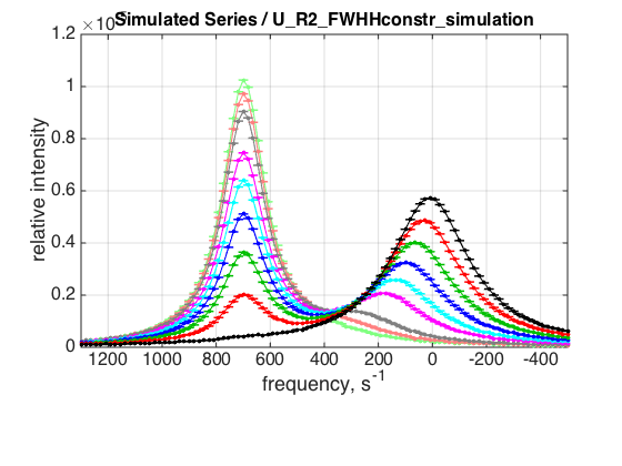
The spectra look completely identical to the simulation with LineShapeKin Simulation 4.1

CONCLUSIONS

The U-R2 model for NMR 1D line shapes works as expected.

Contents