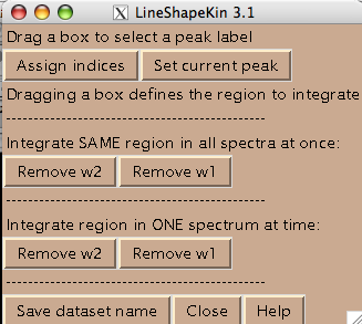
- All spectra in the titration series should have an integer index corresponding to the order in the titration series. Hit [Assign indices]. It brings up new window such as:
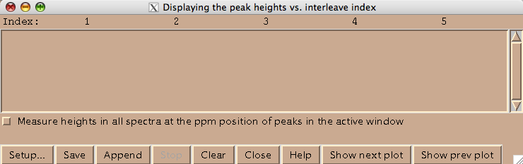
Technically this window belongs to a different Sparky extension (es in Evgenii menu). We invoke it to assign the indices to the 2D planes. Hit [Setup] to open the actual window where you spectra will be listed (both of these windows are based on standard Sparky Python extensions):
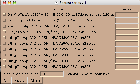
Add integers starting from 1 and click on check-boxes next to the spectra. These are the numbers your titration points will be known to MATLAB as.
(Disregard 'Relative scale...' box. This number is not read by LineShapeKin.)
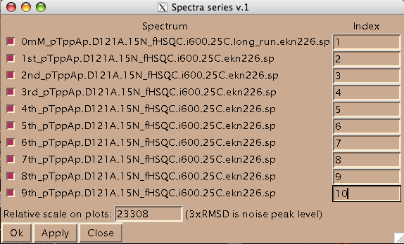
Now you should hit [Apply] and then [Close] to close this window. Hit [Close] in previous window as well and now you are left with just window from LineShapeKin.
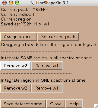
- You are ready to begin extraction of NMR line shapes. First you should select a peak the line shape 1D slices will belong to. Drag a rectangle around the peak label and hit [Set current peak]. The captured peak name is shown in the window.
LineShapeKin will use this name for all 1D slices from now on until you hit [Set current peak] again.
- Next step is to define a region to generate 1D slices. The main way is to look at an overlay of your spectra and drag a rectangle to encompass both free and bound peaks. This is an option 'Integrate SAME region in all spectra at once'. Once you hit [Remove w1] or [Remove w2] LineShapeKin will automatically go through all spectra in the project, extract data, integrate along one dimension to leave w2 or w1, correspondingly, and save them individually for each 2D plane. This is a great way for relatively good S/N datasets with little spectral crowding so you can define a rectangular spectral region where only one peak of interest present throughout entire titration series. Example:
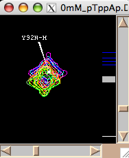
Usually you should define a narrow rectangle going through the peak maxima along the desired dimension so all 1D traces you collect contain significant signal. Once you hit [Remove ...] button LineShapeKin makes a subfolder Data_for_MatLab/Y92N-H_x_w1/ and displays data folder name in Saved as: field.
LineShapeKin output consists of:
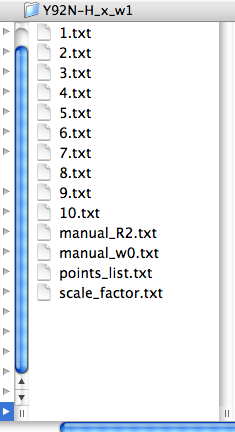
index.txt files with raw integrated spectral data from each spectrum in a plain text form as an X-Y array. This data may be edited. If you prefer, you may produce this kind of data with any other program than Sparky and then read them by LineShapeKin module in MATLAB.
The points_list.txt file that contains a list of indices. This file directs MATLAB LineShapeKin M-notebook to read specific index.txt files so you may exclude any bad titration point from further processing by simply removing corresponding index from this file.
The files manual_R2.txt and manual_w0.txt are produced empty. This is a signal to MATLAB later to initiate automatic estimation of positions and line widths of free and bound state of your molecule. You may override automatic estimates by providing corresponding relaxation rates (/s) or free-, bound- frequencies (Hz) or both.
The file scale_factor.txt contains a numerical factor to scale experimental intensities with for fitting. This factor is applied to all 1D slices so has no influence on the outcome of model fitting. However, different peaks will be sliced differently and yield different total intensities due to integration procedure. To make it possible to do global fitting of multiple residues we need to establish Scale Factors, specific for each peak slicing operation thus making peak intensities for different resonances normalized to unity.
The file is written with '1' but later fitting session in MATLAB allows establishing the correct number to put in here. It is important to remember that the Scale Factor compensates for the specific rectangle you took in Sparky, therefore every new slicing operation will reset the number in the file back to '1' so you have to adjust it again after the first fitting run.
Hit [Set dataset name] to add data set name to the Data_for_MatLab/matlab.peaklist. This is a plain text file generated for your convenience so you could cut-and-paste dataset names from it into the setup.m Matlab notebook.
- Loading this data in MATLAB in 'just display data' mode(see Data analysis in MATLAB)
shows nice array of 1D slices:
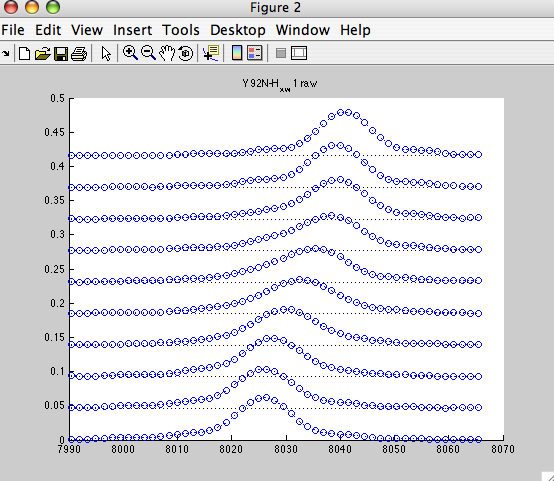
NOTE: the X-axis is following normal direction here. For better comparison with Sparky display you may switch Sparky to Hz units (vt).
- However, nice resolved resonance is not always the case. Frequently we have a neighboring peaks that make using the same rectangle for all spectra impossible. Nice nasty example below:
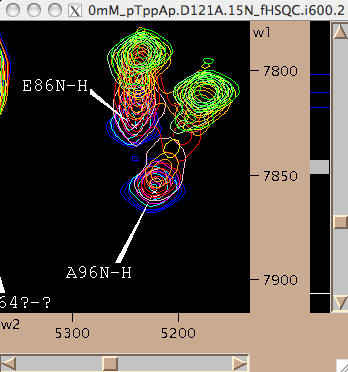
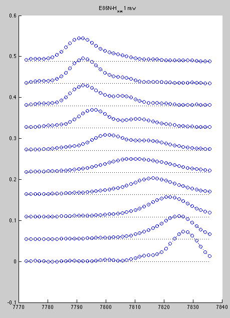
We may slice E86 along w1 like this:
Corresponding line shapes look good:
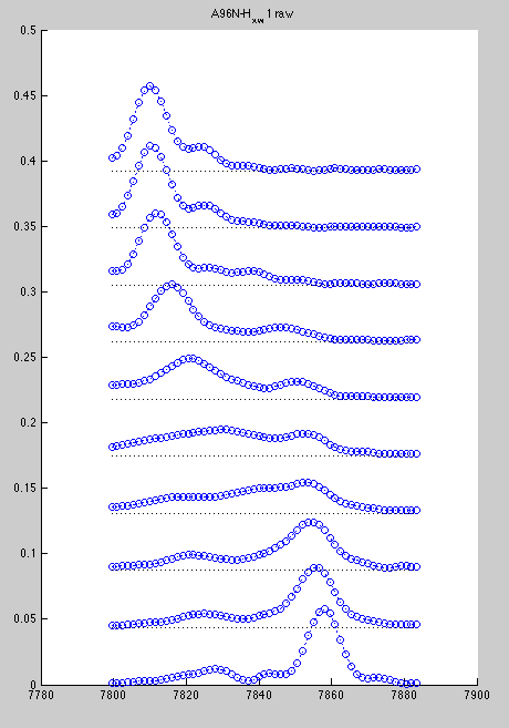
However, A96 is hard to slice if we do all spectra with the same rectangle. Best we can do is this
Here we loose significant intensity from beginning of titration (blue) and get distortion of the end of titration due to E86. Here are resulting line shapes
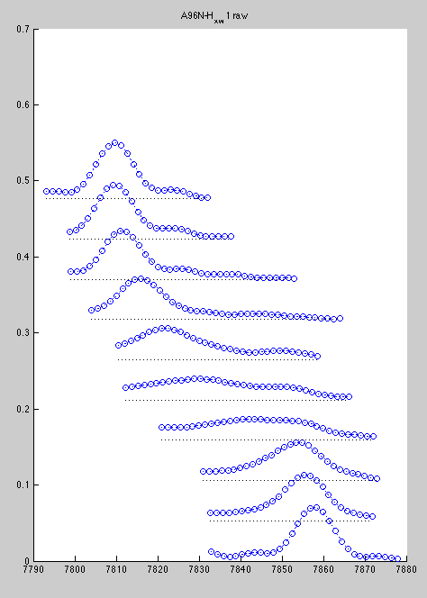
In such a case you can slice one spectrum at a time, because at every titration point two resonances are resolved.
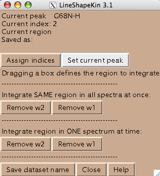
- To do extraction of the line shapes from individual spectra you have to execute 'all spectra at once' option first, because it creates necessary file structure for all spectra. After that, you can draw a rectangle in every individual spectrum and hit [Remove w2] button under the option 'Integrate region in ONE spectrum at a time'. When you do it LineShapeKin replaces the existing 1D slice created from common rectangle ('all spectra at once' option) with the slice using specific current rectangle. The LineShapeKin window will show the index value corresponding to the 2D plane you took data from.
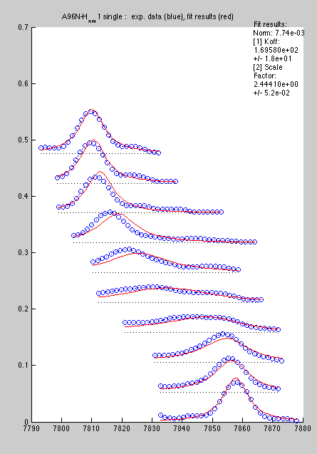
Now line shapes are a bit cleaner than previously and may be fit more reliably:
Certainly, with a large number of peaks to analyze the first procedure is more productive, so I would reserve the second for special cases.