B_R2_R2L2_derivation

B_R2_R2L2

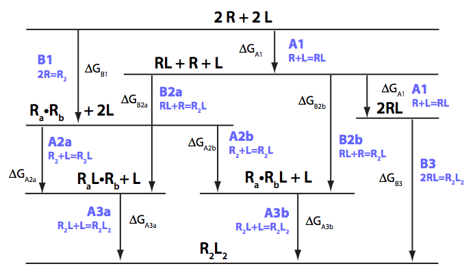
Receptor dimerization coupled with binding of one ligand per receptor monomer

Contents

Goals

1. Definitions

2. Basic equilibrium equations

3. Analysis of statistical effects on binding constants

4. Derivation of equations for concentrations of species in terms of MACROSCOPIC constants

Summary of equations for equilibrium concentrations and relationship to MICROSCOPIC constants

5. Prepare equations for a numeric solution in MICROSCOPIC constants

6. Save results on disk for future use

Conclusions

Back to Contents

Goals

In this notebook I will derive equations for binding of a ligand to a receptor molecule coupled with dimerization of the receptor and prepare equations for numerical simulations.

Analysis will be done in

EKM16.Analysis_of_multistep_kinetic_mechanisms/Equilibria/B-R2-R2L2_model/B_R2_R2L2_analysis.mn

Back to Contents

1. Definitions

clean up workspace

reset()

Set path to save results into:

ProjectName:="B_R2_R2L2";

CurrentPath:="/Users/kovrigin/Documents/Workspace/Data/Data.XV/EKM16.Analysis_of_multistep_kinetic_mechanisms/Equilibria/B_R2_R2L2_model/";

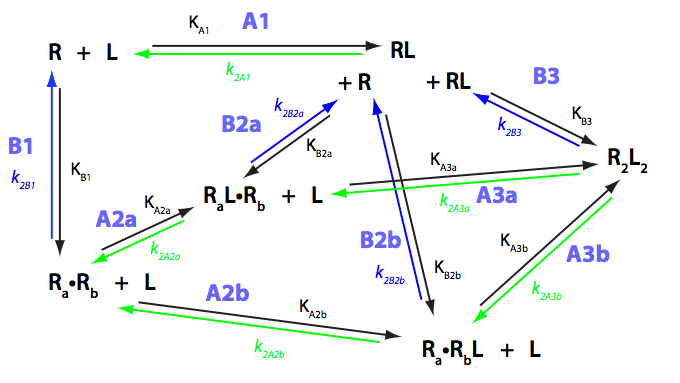
We need to consider the system two ways: using macroscopic and microscopic binding constants [1]. Overall, these are two completely equivalent treatments but interpretation in terms of mechanistic events is only available for microscopic constants. We are especially interested in microscopic constants because we may assess cooperativity between the sites.

Symmetry of the system makes it easy to use macroscopic treatment and simply substitute microscopic constants into it.

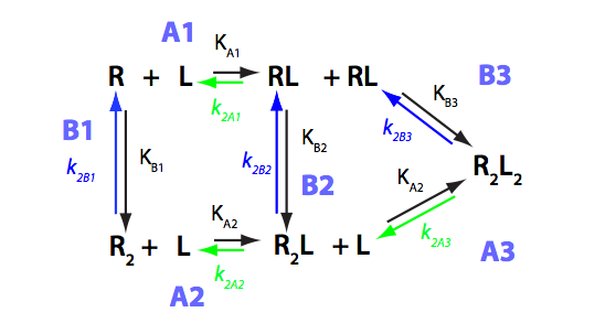
Binding and isomerization constants

All binding constants I am using are association constants.

These relationships serve as restraints for solve(), but not restrict these values in calculations!

Macroscopic constants

K_A_1

K_A_1 ;

assumeAlso(K_A_1 > 0):

assumeAlso(K_A_1 , R_):

K_A_2

K_A_2 ;

assumeAlso(K_A_2 > 0):

assumeAlso(K_A_2 , R_):

K_A_3

K_A_3 ;

assumeAlso(K_A_3 > 0):

assumeAlso(K_A_3 , R_):

K_B_1

K_B_1 ;

assumeAlso(K_B_1 > 0):

assumeAlso(K_B_1 , R_):

K_B_2

K_B_2 ;

assumeAlso(K_B_2 > 0):

assumeAlso(K_B_2 , R_):

K_B_3

K_B_3 ;

assumeAlso(K_B_3 > 0):

assumeAlso(K_B_3 , R_):

Microscopic constants

KB2micro

K_B_2_m;

assumeAlso(K_B_2_m > 0):

assumeAlso(K_B_2_m , R_):

KA2micro

K_A_2_m;

assumeAlso(K_A_2_m > 0):

assumeAlso(K_A_2_m , R_):

KA3micro

K_A_3_m;

assumeAlso(K_A_3_m > 0):

assumeAlso(K_A_3_m , R_):

Total concentrations

Rtot - total concentration of the receptor

Rtot;

assumeAlso(Rtot>0):

assumeAlso(Rtot,R_):

Ltot - total concentration of a ligand

Ltot;

assumeAlso(Ltot>0):

assumeAlso(Ltot,R_):

Equilibrium concentrations

Req

Req;

assumeAlso(Req>0):

assumeAlso(Req<Rtot):

assumeAlso(Req,R_):

Leq

Leq;

assumeAlso(Leq>0):

assumeAlso(Leq<Ltot):

assumeAlso(Leq,R_):

RLeq

RLeq;

assumeAlso(RLeq>0):

assumeAlso(RLeq<Rtot):

assumeAlso(RLeq<Ltot):

assumeAlso(RLeq,R_):

R2eq

R2eq;

assumeAlso(R2eq>0):

assumeAlso(R2eq<Rtot/2):

assumeAlso(R2eq,R_):

R2Leq

R2Leq;

assumeAlso(R2Leq>0):

assumeAlso(R2Leq<Rtot/2):

assumeAlso(R2Leq<Ltot):

assumeAlso(R2Leq,R_):

R2L2eq

R2L2eq;

assumeAlso(R2L2eq>0):

assumeAlso(R2L2eq<Rtot/2):

assumeAlso(R2L2eq<Ltot/2):

assumeAlso(R2L2eq,R_):

Microscopic species

R2Laeq;

assumeAlso(R2Laeq>0):

assumeAlso(R2Laeq<Rtot/2):

assumeAlso(R2Laeq<Ltot):

assumeAlso(R2Laeq,R_):

R2Lbeq;

assumeAlso(R2Lbeq>0):

assumeAlso(R2Lbeq<Rtot/2):

assumeAlso(R2Lbeq<Ltot):

assumeAlso(R2Lbeq,R_):

anames(Properties,User);

math

Back to Contents

2. Basic equilibrium equations

Working equation: I will try to express analytical [L] from equation for a total concentration of a receptor or use the expression for a numeric solution if analytical is not possible.

Total concentrations of a receptor and a ligand

eq2_1:= Rtot = Req + RLeq + 2*R2eq + 2*R2Leq + 2*R2L2eq;

eq2_2:= Ltot = Leq + RLeq + R2Leq + 2*R2L2eq;

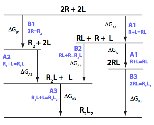
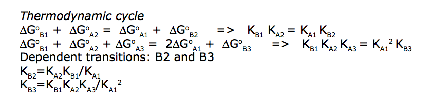
Write equilibrium thermodynamics equations using macroscopic constants (KB2 and KB3 are chosen to be dependent constants).

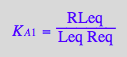
eq2_3:= K_A_1 = RLeq / (Req*Leq);

math

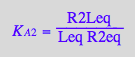
eq2_4:= K_A_2 = R2Leq / (R2eq*Leq);

math

eq2_5:= K_A_3 = R2L2eq / (R2Leq*Leq);

math

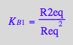
eq2_6:= K_B_1 = R2eq / (Req*Req);

math

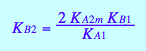
eq2_7:= K_B_2 = R2Leq / (RLeq*Req);

math

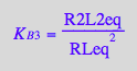
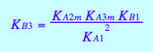
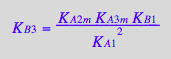
eq2_8:= K_B_3 = R2L2eq / (RLeq*RLeq);

math

Write additional equilibrium equations defining microscopic constants and species

eq2_9:= R2Leq = R2Laeq + R2Lbeq

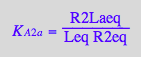
eq2_10:= K_A_2_a = R2Laeq / (R2eq*Leq)

math

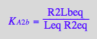
eq2_11:= K_A_2_b = R2Lbeq / (R2eq*Leq)

math

eq2_12:= K_A_3_a = R2L2eq / (R2Laeq*Leq)

math

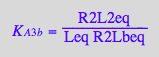
eq2_13:= K_A_3_b = R2L2eq / (R2Lbeq*Leq)

math

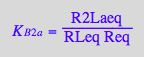
eq2_14:= K_B_2_a = R2Laeq / (RLeq*Req)

math

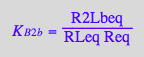
eq2_15:= K_B_2_b = R2Lbeq / (RLeq*Req)

math

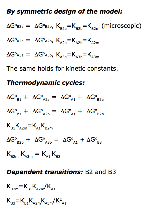
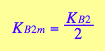
Equalities for microscopic constants due to symmetry of the model:

eq2_16:= K_B_2_a = K_B_2_m;

eq2_17:= K_B_2_b = K_B_2_m;

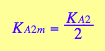
eq2_18:= K_A_2_a = K_A_2_m;

eq2_19:= K_A_2_b = K_A_2_m;

eq2_20:= K_A_3_a = K_A_3_m;

eq2_21:= K_A_3_b = K_A_3_m;

Back to Contents

3. Analysis of statistical effects on binding constants

Establish relationship between microscopic and macroscopic binding constants

B2 transition

R2Laeq

eq2_14;

solve(%,R2Laeq);

%[1][1];

eq3_1:= R2Laeq = %

math

R2Lbeq

eq2_15;

solve(%,R2Lbeq);

%[1][1];

eq3_2:= R2Lbeq = %

math

Substitute to mass conservation law

eq2_9;

% | eq3_1 | eq3_2;

eq3_3:= %:

Substitute in K_B_2 expression

eq2_7;

% | eq3_3;

normal(%);

% | eq2_16 | eq2_17;

eq3_4a:= %:

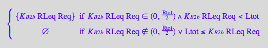
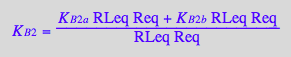
solve(%,K_B_2_m);

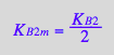
eq3_4b:= K_B_2_m = %[1]

math

A2 transition

R2Laeq

eq2_10;

solve(%,R2Laeq);

%[1][1];

eq3_5:= R2Laeq = %;

math

R2Lbeq

eq2_11;

solve(%,R2Lbeq);

%[1][1];

eq3_6:= R2Lbeq = %

math

Mass conservation

eq2_9;

% | eq3_5 | eq3_6;

eq3_7:= %:

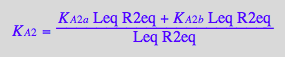
Substitute into macroscopic constant equation

eq2_4;

% | eq3_7 ;

% | eq2_18 | eq2_19;

eq3_9a:= %:

solve(%,K_A_2_m);

eq3_9b:= K_A_2_m = %[1]

math

A3 transition

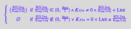
R2Laeq

eq2_12;

solve(%,R2Laeq);

%[1][1];

eq3_10:= R2Laeq = %

math

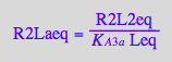
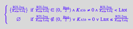
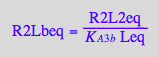
R2Lbeq

eq2_13;

solve(%, R2Lbeq);

%[1][1];

eq3_11:= R2Lbeq = %

math

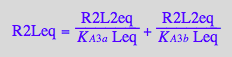
Mass conservation

eq2_9;

% | eq3_10 | eq3_11;

eq3_12:= %:

math

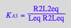
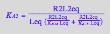
Substitute into the macroscopic constants equation

eq2_5;

% | eq3_12;

% | eq2_20 | eq2_21;

eq3_13a:= %:

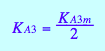
solve(%,K_A_3_m);

eq3_13b:= K_A_3_m = %[1]

math

Relationships between kinetic and equilibrium constants

A2 transition

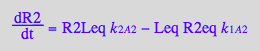
Macro:

dR2/dt = -k_1_A_2*R2eq*Leq + k_2_A_2*R2Leq

math

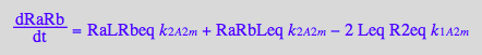
Micro:

dRaRb/dt = -2*k_1_A_2_m*R2eq*Leq + k_2_A_2_m*RaLRbeq +k_2_A_2_m*RaRbLeq

math

dRaRb/dt= -2*k_1_A_2_m*R2eq*Leq + k_2_A_2_m*R2Leq

math

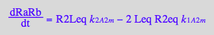
Comparing first and last equation we can equate:

eq3_20:= k_2_A_2_m=k_2_A_2

eq3_21:= 2*k_1_A_2_m=k_1_A_2

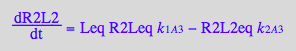
A3 transition

Macro:

dR2L2/dt = k_1_A_3*R2Leq*Leq - k_2_A_3*R2L2eq

math

Micro:

dR2L2/dt = -2*k_2_A_3_m*R2L2eq + k_1_A_3_m*RaLRbeq*Leq +k_1_A_3_m*RaRbLeq*Leq

math

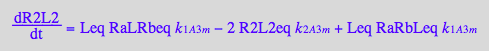
dR2L2/dt= -2*k_2_A_3_m*R2L2eq + k_1_A_3_m*R2Leq*Leq

math

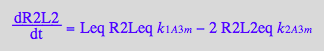
Comparing first and last equations we can equate:

eq3_22:= k_1_A_3_m=k_1_A_3

eq3_23:= 2*k_2_A_3_m=k_2_A_3

Summary of relationships between

micro- and macroscopic equilibrium binding constants

eq3_4a; eq3_4b;

math

eq3_9a; eq3_9b

math

eq3_13a; eq3_13b

math

Relationships of kinetic constants

eq3_20;

eq3_21

eq3_22

eq3_23

Back to Contents

4. Derivation of equations for concentrations of species in terms of MACROSCOPIC constants

Express Leq as a function of macroscopic constants and total concentrations of a receptor and a ligand

Independent equations to use:

eq2_1;eq2_2

eq2_3;eq2_4;eq2_5;eq2_6;eq3_9a;eq3_13a

math

Express complex species concentrations:

RLeq

eq2_3;

solve(%,RLeq);

%[1][1];

eq4_1:= RLeq = %

math

R2eq

eq2_6;

solve(%,R2eq);

%[1][1];

eq4_2:= R2eq = %

math

R2Leq

eq2_4;

% | eq4_2;

solve(%,R2Leq);

%[1][1];

eq4_3:= R2Leq = % | eq3_9a

math

R2L2eq

eq2_5;

% | eq4_3;

solve(%, R2L2eq);

%[1][1];

eq4_4:= R2L2eq = % | eq3_13a

math

Substitute into a mass conservation law for L and express Req

eq2_2;

% | eq4_4;

% | eq4_3;

% | eq4_1;

eq4_5:= %:

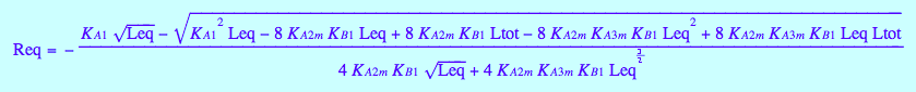
Solve for Req

solutions4_5:=solve(eq4_5,Req):

eq4_6:= solutions4_5[i,1] $ i=1..nops(solutions4_5):

print(Unquoted,"Number of formal solutions: ".nops(%))

Number of formal solutions: 4

How many independent soltions we have?

Is 1st solution a combination of 2nd and 3rd?

solution1:=eq4_6[1]; // a sequence of roots (multiple solutions)

solution2:=eq4_6[2][1]; // extract equation out of a sequence

solution3:=eq4_6[3][1]; // extract equation out of a sequence

if solution2 in solution1

then print(Unquoted,"First set of roots contains the second root.");

else print(Unquoted,"First set of roots DOES NOT contain the second root!");

end_if;

if solution3 in solution1

then print(Unquoted,"First set of roots contains the third root.");

else print(Unquoted,"First set of roots DOES NOT contain the third root!");

end_if;

math

First set of roots contains the second root.

First set of roots contains the third root.

Check correctness of the solutions by substitution into original equation solved:

Check first root

test1:= eq4_5 | Req=solution2:

normal(%);

Check the second root

test2:= eq4_5 | Req=solution3:

normal(%);

Both solutions are correct.

Choose meaningful one for further work

solution2 | Rtot=1 | Ltot=0.1 | Leq=0.001 | K_A_1=1 | K_B_1=1 | K_A_2_m=1 | K_A_3_m=1

solution3 | Rtot=0.1 | Ltot=0.1 | Leq=0.01 | K_A_1=1 | K_B_1=1 | K_A_2_m=1 | K_A_3_m=1

Solution 2 is meaningful !

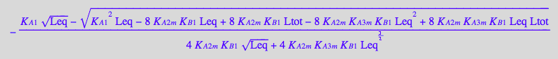
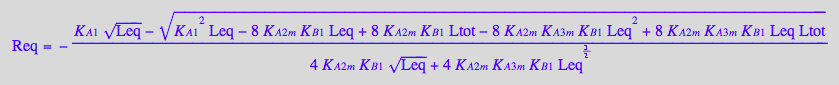
ASSIGN TO AN EQUATION:

eq4_7:= Req = solution2;

math

Finally, substitute all into a mass conservation law for a receptor

eq2_1;

% | eq4_1 | eq4_2 | eq4_3 | eq4_4 ;

% | eq4_7;

eq4_8:= %:

math

Check consistency: derive equations for dependent constants

Kb2

eq2_7 ;

% | eq4_3 | eq4_1 ;

solve(%,K_B_2);

eq4_9:= K_B_2 =%[1]

math

Correct.

KB3

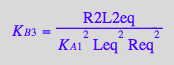
eq2_8;

% | eq4_1;

% | eq4_4;

eq4_10:= %:

math

Summary of equations for equilibrium concentrations

Independent parameters:

Rtot, Ltot, K_A_1, K_B_1, K_A_2, K_A_3

Macroscopic constants in terms of microscopic ones:

eq3_9a

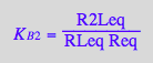
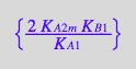
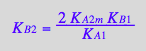
eq3_4a

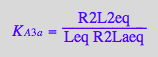
eq3_13a

math

Relationships of kinetic constants

eq3_20;

eq3_21

eq3_22

eq3_23

Equation to solve:

Rtot=f([L])

eq4_8

math

Equilibrium concentrations of species:

[R]

eq4_7

math

[RL]

eq4_1

[R2]

eq4_2

[R2L]

eq4_3

[R2L2]

eq4_4

Dependent equilibrium constants

eq4_9

math

eq4_10

math

Back to Contents

5. Prepare equations for a numeric solution in MICROSCOPIC constants

I will express all equilibrium concentrations in terms of each other in successive order, easy to code in Matlab.

Make a function for numeric solving and switch to LRratio=Ltot/Rtot

eq5_1:= Ltot=LRratio*Rtot;

fRtot_B_R2_R2L2:=(Rtot, LRratio, Leq, K_A_1, K_B_1, K_A_2_m, K_A_3_m) --> eq4_8[2] | eq5_1;

math

Assume some constant values for testing

Total_R:=1e-3:

Ka1:=1e7:

Kb1:=2e3:

Ka2m:=1e5:

Ka3m:=1e5:

LR_Ratio_max:=2.5:

LR_Ratio:=0.8:

Test fRtot:

fRtot_B_R2_R2L2(Total_R, LR_Ratio, 1e-4, Ka1, Kb1, Ka2m, Ka3m)

it works OK.

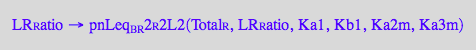
Define a procedure for numeric solving the equation Rtot=f([L]) for [L] thus creating a function [L]=f(Rtot,...)

// WARNING: make sure the Leq search range starts with a non-zero number!!!! Use a number larger than that to create approximation of LRratio=0

pnLeq_B_R2_R2L2:= proc(Total_R, LR_Ratio, Ka1, Kb1, Ka2m, Ka3m)

/* Parameter names should be different from

variable names used in the equation!!!

If you see an error message:

"Error: Illegal operand [_index];

during evaluation of 'your function name'"

it means fsolve() returned FAIL and you need to check

values of all parameters passed to the function fRtot

local result, L;

begin

//print(Total_R, LR_Ratio, Ka1, Kb1, Ka2m, Ka3m);

// numeric solving equation for Leq in a restricted range.

// WARNING: make sure the range starts with a non-zero number!!!!

result:=numeric::fsolve(

Total_R=fRtot_B_R2_R2L2(Total_R, LR_Ratio, Leq, Ka1, Kb1, Ka2m, Ka3m),

Leq=10e-32..Total_R*LR_Ratio);

//print(result);

// extract answer from equation

L:=result[1][2];

//print(Unquoted,"solve() residual: ".(Total_R-fRtot_B_R2_R2L2(Total_R, LR_Ratio, L, Ka1, Kb1, Ka2m, Ka3m)));

return(L);

end_proc;

test operation

Total_R:=1:

Ka1:=1e7:

Kb1:=2e3:

Ka2m:=1e5:

Ka3m:=1e5:

LR_Ratio_max:=2.5:

LR_Ratio:=10:

DIGITS:=10;

pnLeq_B_R2_R2L2(Total_R, LR_Ratio, Ka1, Kb1, Ka2m, Ka3m) ;

Make "portable" equations

(unique names for future use):

eq3_9a

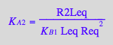
eq3_4a

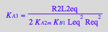
eq3_13a

math

RLeq_B_R2_R2L2:=eq4_1;

R2eq_B_R2_R2L2:=eq4_2;

R2Leq_B_R2_R2L2:=eq4_3;

R2L2eq_B_R2_R2L2:=eq4_4;

Req_B_R2_R2L2:=eq4_7;

Rtot_B_R2_R2L2:=eq4_8:

KB2_B_R2_R2L2:=eq4_9;

KB3_B_R2_R2L2:=eq4_10;

KA2_B_R2_R2L2:=eq3_9a;

KB2_B_R2_R2L2:=eq3_4a;

KA3_B_R2_R2L2:=eq3_13a;

math

Define functions for equilibrium concentrations of all species:

[R]

Req_B_R2_R2L2;

pnReq_B_R2_R2L2:= proc(Total_R, LR_Ratio, Ka1, Kb1, Ka2m, Ka3m)

// Parameter names should be different from

// variable names used in the equation!!!

local L;

begin

L:=pnLeq_B_R2_R2L2(Total_R, LR_Ratio, Ka1, Kb1, Ka2m, Ka3m);

// Equation for [R]

end_proc

math

test

Total_R:=1:

Ka1:=10:

Kb1:=1e3:

Ka2m:=1:

Ka3m:=1:

LR_Ratio_min:=1e-2:

LR_Ratio_max:=10:

pnReq_B_R2_R2L2(Total_R, LR_Ratio_min, Ka1, Kb1, Ka2m, Ka3m) ;

pnReq_B_R2_R2L2(Total_R, LR_Ratio_max, Ka1, Kb1, Ka2m, Ka3m) ;

Total_R:=1:

Ka1:=1.0:

Ka2m:=10.0:

Ka3m:=100.0:

Kb1:=0.1:

LR_Ratio_min:=0.1:

LR_Ratio_max:=1:

pnReq_B_R2_R2L2(Total_R, LR_Ratio_min, Ka1, Kb1, Ka2m, Ka3m) ;

[RL]

RLeq_B_R2_R2L2;

pnRLeq_B_R2_R2L2:= proc(Total_R, LR_Ratio, Ka1, Kb1, Ka2m, Ka3m)

// Parameter names should be different from

// variable names used in the equation!!!

local L, R;

begin

L:=pnLeq_B_R2_R2L2(Total_R, LR_Ratio, Ka1, Kb1, Ka2m, Ka3m);

R:=pnReq_B_R2_R2L2(Total_R, LR_Ratio, Ka1, Kb1, Ka2m, Ka3m);

// Equation for [R]

end_proc

test

pnRLeq_B_R2_R2L2(Total_R, LR_Ratio_min, Ka1, Kb1, Ka2m, Ka3m) ;

pnRLeq_B_R2_R2L2(Total_R, LR_Ratio_max, Ka1, Kb1, Ka2m, Ka3m) ;

[R2]

R2eq_B_R2_R2L2;

pnR2eq_B_R2_R2L2:= proc(Total_R, LR_Ratio, Ka1, Kb1, Ka2m, Ka3m)

// Parameter names should be different from

// variable names used in the equation!!!

local L, R;

begin

R:=pnReq_B_R2_R2L2(Total_R, LR_Ratio, Ka1, Kb1, Ka2m, Ka3m);

// Equation for [R]

end_proc

test

pnR2eq_B_R2_R2L2(Total_R, LR_Ratio_min, Ka1, Kb1, Ka2m, Ka3m) ;

pnR2eq_B_R2_R2L2(Total_R, LR_Ratio_max, Ka1, Kb1, Ka2m, Ka3m) ;

[R2L]

R2Leq_B_R2_R2L2;

pnR2Leq_B_R2_R2L2:= proc(Total_R, LR_Ratio, Ka1, Kb1, Ka2m, Ka3m)

// Parameter names should be different from

// variable names used in the equation!!!

local L, R;

begin

L:=pnLeq_B_R2_R2L2(Total_R, LR_Ratio, Ka1, Kb1, Ka2m, Ka3m);

R:=pnReq_B_R2_R2L2(Total_R, LR_Ratio, Ka1, Kb1, Ka2m, Ka3m);

// Equation for [R]

end_proc

test

pnR2Leq_B_R2_R2L2(Total_R, LR_Ratio_min, Ka1, Kb1, Ka2m, Ka3m) ;

pnR2Leq_B_R2_R2L2(Total_R, LR_Ratio_max, Ka1, Kb1, Ka2m, Ka3m) ;

[R2L2]

R2L2eq_B_R2_R2L2;

pnR2L2eq_B_R2_R2L2:= proc(Total_R, LR_Ratio, Ka1, Kb1, Ka2m, Ka3m)

// Parameter names should be different from

// variable names used in the equation!!!

local L, R;

begin

L:=pnLeq_B_R2_R2L2(Total_R, LR_Ratio, Ka1, Kb1, Ka2m, Ka3m);

R:=pnReq_B_R2_R2L2(Total_R, LR_Ratio, Ka1, Kb1, Ka2m, Ka3m);

// Equation for [R]

end_proc

test

Total_R:=1:

Ka1:=10:

Kb1:=1e3:

Ka2m:=1:

Ka3m:=1:

LR_Ratio:=8:

pnR2L2eq_B_R2_R2L2(Total_R, LR_Ratio, Ka1, Kb1, Ka2m, Ka3m);

LR_Ratio:=10:

pnR2L2eq_B_R2_R2L2(Total_R, LR_Ratio, Ka1, Kb1, Ka2m, Ka3m);

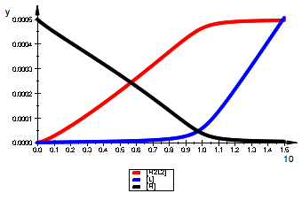
Test plotting

Total_R:=1e-3:

Ka1:=10:

Kb1:=1e3:

Ka2m:=1e5:

Ka3m:=1e6:

LR_Ratio_min:=1E-16:

LR_Ratio_max:=1.5:

pnR2L2eq_B_R2_R2L2(Total_R, LR_Ratio_min, Ka1, Kb1, Ka2m, Ka3m);

pnR2L2eq_B_R2_R2L2(Total_R, LR_Ratio_max, Ka1, Kb1, Ka2m, Ka3m);

// Make wrapper functions dependent on LRratio

fnLeq:=LR_Ratio -> pnLeq_B_R2_R2L2(Total_R, LR_Ratio, Ka1, Kb1, Ka2m, Ka3m) ;

fnReq:=LR_Ratio -> pnReq_B_R2_R2L2(Total_R, LR_Ratio, Ka1, Kb1, Ka2m, Ka3m) :

fnRLeq:=LR_Ratio -> pnRLeq_B_R2_R2L2(Total_R, LR_Ratio, Ka1, Kb1, Ka2m, Ka3m) :

fnR2eq:=LR_Ratio -> pnR2eq_B_R2_R2L2(Total_R, LR_Ratio, Ka1, Kb1, Ka2m, Ka3m) :

fnR2Leq:=LR_Ratio -> pnR2Leq_B_R2_R2L2(Total_R, LR_Ratio, Ka1, Kb1, Ka2m, Ka3m) :

fnR2L2eq:=LR_Ratio -> pnR2L2eq_B_R2_R2L2(Total_R, LR_Ratio, Ka1, Kb1, Ka2m, Ka3m) :

print(Unquoted,"Leq ",fnLeq(LR_Ratio_min),fnLeq(LR_Ratio_max));

print(Unquoted,"Req ",fnReq(LR_Ratio_min),fnReq(LR_Ratio_max));

print(Unquoted,"RLeq ",fnLeq(LR_Ratio_min),fnRLeq(LR_Ratio_max));

print(Unquoted,"R2eq ",fnR2eq(LR_Ratio_min),fnR2eq(LR_Ratio_max));

print(Unquoted,"R2Leq ",fnR2Leq(LR_Ratio_min),fnR2Leq(LR_Ratio_max));

print(Unquoted,"R2L2eq ",fnR2L2eq(LR_Ratio_min),fnR2L2eq(LR_Ratio_max));

LW:=1.5:

pLeq:= plot::Function2d(

Function=(fnLeq),

LegendText="[L]",

Color = RGB::Blue,

XMin=(LR_Ratio_min),

XMax=(LR_Ratio_max),

XName=(LR_Ratio),

TitlePositionX=(0),

LineWidth=LW):

pReq:= plot::Function2d(

Function=(fnReq),

LegendText="[R]",

Color = RGB::Black,

XMin=(LR_Ratio_min),

XMax=(LR_Ratio_max),

XName=(LR_Ratio),

TitlePositionX=(0),

LineWidth=LW):

pR2L2eq:= plot::Function2d(

Function=(fnR2L2eq),

LegendText="[R2L2]",

Color = RGB::Red,

XMin=(LR_Ratio_min),

XMax=(LR_Ratio_max),

XName=(LR_Ratio),

TitlePositionX=(0),

LineWidth=LW):

plot(pR2L2eq,pLeq,pReq,LegendVisible=TRUE);

math

Leq , 1.960592105e-21, 0.0005063940189

Req , 0.0004999999992, 0.000004397139854

RLeq , 1.960592105e-21, 0.00000002226685322

R2eq , 0.0002499999992, 0.0000000193348389

R2Leq , 9.802960493e-20, 0.000001958209355

R2L2eq , 9.609803474e-35, 0.0004958127525

MuPAD graphics

Back to Contents

6. Save results on disk for future use

(you can retrieve them later by executing: fread(filename,Quiet))

ProjectName;

CurrentPath

Save all numeric solutions:

filename:=CurrentPath.ProjectName.".mb";

write(filename,

// save basic equations

fRtot_B_R2_R2L2,

Req_B_R2_R2L2,

R2eq_B_R2_R2L2,

RLeq_B_R2_R2L2,

R2Leq_B_R2_R2L2,

R2L2eq_B_R2_R2L2,

// save dependent constants

KB2_B_R2_R2L2,

KB3_B_R2_R2L2,

// constants in terms of microscopic constants

KA2_B_R2_R2L2,

KB2_B_R2_R2L2,

KA3_B_R2_R2L2,

// save numeric procedures

pnLeq_B_R2_R2L2,

pnReq_B_R2_R2L2,

pnR2eq_B_R2_R2L2,

pnRLeq_B_R2_R2L2,

pnR2Leq_B_R2_R2L2,

pnR2L2eq_B_R2_R2L2

)

Relationships between kinetic constants

Conclusions

1. This system is analytically insoluble.

2. I derived numeric solutions in MACROSCOPIC constants and saved them.

3. Line shape and any kinetic simulations must be done with microscopic constants.

Back to Contents