U-5R
Derivation of equilibrium thermodynamic equations for U-5R system: isomerization in the binding-incompetent state of the receptor (many states)
Here I will analyze numeric solutions I derived in U_2R_derivation.mn.
Clean up
reset()
Path to previous results
ProjectName:="U-5R";
CurrentPath:="/Users/kovrigin_laptop/Documents/Workspace/Global_Analysis/IDAP/Mathematical_models/Equilibrium_thermodynamic_models/U-multi-path-models/nR/U-5R";
![]()

Read results of derivations
filename:=CurrentPath."/".ProjectName.".mb";
fread(filename,Quiet):
anames(User)


Assume some values for testing operation
Total_R:=1e-3:
Total_L:=10e-3:
Ka:=1e3:
Kb_s1:=2:
Kb_s2:=3:
Kb_s3:=4:
Kb_s4:=5:
Kb_s5:=6:
test operation of all functions
fLeq_U_5R(Total_R, Total_L, Ka, Kb_s1, Kb_s2, Kb_s3, Kb_s4, Kb_s5);
fReq_U_5R(Total_R, Total_L, Ka, Kb_s1, Kb_s2, Kb_s3, Kb_s4, Kb_s5);
fR_s_1eq_U_5R(Total_R, Total_L, Ka, Kb_s1, Kb_s2, Kb_s3, Kb_s4, Kb_s5);
fR_s_2eq_U_5R(Total_R, Total_L, Ka, Kb_s1, Kb_s2, Kb_s3, Kb_s4, Kb_s5);
fR_s_3eq_U_5R(Total_R, Total_L, Ka, Kb_s1, Kb_s2, Kb_s3, Kb_s4, Kb_s5);
fR_s_4eq_U_5R(Total_R, Total_L, Ka, Kb_s1, Kb_s2, Kb_s3, Kb_s4, Kb_s5);
fR_s_5eq_U_5R(Total_R, Total_L, Ka, Kb_s1, Kb_s2, Kb_s3, Kb_s4, Kb_s5);
fRLeq_U_5R(Total_R, Total_L, Ka, Kb_s1, Kb_s2, Kb_s3, Kb_s4, Kb_s5);
![]()
![]()
![]()
![]()
![]()
![]()
![]()
![]()
=> operative
Make wrapper functions for plotting using L/R as X axis
fLeq:=LRratio -> fLeq_U_5R (Total_R, LRratio*Total_R, Ka, Kb_s1, Kb_s2, Kb_s3, Kb_s4, Kb_s5):
fReq:=LRratio -> fReq_U_5R (Total_R, LRratio*Total_R, Ka, Kb_s1, Kb_s2, Kb_s3, Kb_s4, Kb_s5):
fR_s_1eq:=LRratio -> fR_s_1eq_U_5R (Total_R, LRratio*Total_R, Ka, Kb_s1, Kb_s2, Kb_s3, Kb_s4, Kb_s5):
fR_s_2eq:=LRratio -> fR_s_2eq_U_5R (Total_R, LRratio*Total_R, Ka, Kb_s1, Kb_s2, Kb_s3, Kb_s4, Kb_s5):
fR_s_3eq:=LRratio -> fR_s_3eq_U_5R (Total_R, LRratio*Total_R, Ka, Kb_s1, Kb_s2, Kb_s3, Kb_s4, Kb_s5):
fR_s_4eq:=LRratio -> fR_s_4eq_U_5R (Total_R, LRratio*Total_R, Ka, Kb_s1, Kb_s2, Kb_s3, Kb_s4, Kb_s5):
fR_s_5eq:=LRratio -> fR_s_5eq_U_5R (Total_R, LRratio*Total_R, Ka, Kb_s1, Kb_s2, Kb_s3, Kb_s4, Kb_s5):
fRLeq:=LRratio -> fRLeq_U_5R (Total_R, LRratio*Total_R, Ka, Kb_s1, Kb_s2, Kb_s3, Kb_s4, Kb_s5):
Test plotting
Total_R:=1e-3:
LRratio_max:=2:
Ka:=1e6:
Kb_s1:=2:
Kb_s2:=3:
Kb_s3:=4:
Kb_s4:=5:
Kb_s5:=6:
LineW:=1.5: //line width
// create plots
pLeq:= plot::Function2d(
Function=(fLeq),
LegendText="[L]",
Color = RGB::Blue,
XMin=(0),
XMax=(LRratio_max),
XName=(LRratio),
TitlePositionX=(0),
LineWidth=LineW):
pRLeq:= plot::Function2d(
Function=(fRLeq),
LegendText="[RL]",
Color = RGB::Red,
XMin=(0),
XMax=(LRratio_max),
XName=(LRratio),
TitlePositionX=(0),
LineWidth=LineW):
plot(pLeq, pRLeq, LegendVisible=TRUE)
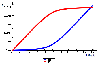
=> works
Assume some constants and evaluate titrations.
NOTE: Adjust dependent constant calculation if necessary.
Simulation_name:= "Full model":
Total_R:=1e-3:
LRratio_max:=2:
Ka:=1e6:
Kb_s1:=2:
Kb_s2:=3:
Kb_s3:=4:
Kb_s4:=5:
Kb_s5:=6:
LRratio_max:=1.5: // plotting range
LineW:=1.5: // plot line width
pLeq:= plot::Function2d(
Function=(fLeq),
LegendText="[L]",
Color = RGB::Blue,
XMin=(LRratio_max*1e-6),
XMax=(LRratio_max),
XName=(LRratio),
TitlePositionX=(0),
LineWidth=LineW):
pReq:= plot::Function2d(
Function=(fReq),
LegendText="[R]",
Color = RGB::Black,
XMin=(LRratio_max*1e-6),
XMax=(LRratio_max),
XName=(LRratio),
TitlePositionX=(0),
LineWidth=LineW):
pR_s_1eq:= plot::Function2d(
Function=(fR_s_1eq),
LegendText="[R*]",
Color = RGB::Green,
XMin=(LRratio_max*1e-6),
XMax=(LRratio_max),
XName=(LRratio),
TitlePositionX=(0),
LineWidth=LineW):
pR_s_2eq:= plot::Function2d(
Function=(fR_s_2eq),
LegendText="[R**]",
Color = RGB::Grey,
XMin=(LRratio_max*1e-6),
XMax=(LRratio_max),
XName=(LRratio),
TitlePositionX=(0),
LineWidth=LineW):
pR_s_3eq:= plot::Function2d(
Function=(fR_s_3eq),
LegendText="[R***]",
Color = RGB::Magenta,
XMin=(LRratio_max*1e-6),
XMax=(LRratio_max),
XName=(LRratio),
TitlePositionX=(0),
LineWidth=LineW):
pR_s_4eq:= plot::Function2d(
Function=(fR_s_4eq),
LegendText="[R****]",
Color = RGB::Yellow,
XMin=(LRratio_max*1e-6),
XMax=(LRratio_max),
XName=(LRratio),
TitlePositionX=(0),
LineWidth=LineW):
pR_s_5eq:= plot::Function2d(
Function=(fR_s_5eq),
LegendText="[R*****]",
Color = RGB::Cyan,
XMin=(LRratio_max*1e-6),
XMax=(LRratio_max),
XName=(LRratio),
TitlePositionX=(0),
LineWidth=LineW):
pRLeq:= plot::Function2d(
Function=(fRLeq),
LegendText="[RL]",
Color = RGB::Red,
XMin=(LRratio_max*1e-6),
XMax=(LRratio_max),
XName=(LRratio),
TitlePositionX=(0),
LineWidth=LineW):
// Text report
print(Unquoted, Simulation_name);
print(Unquoted,"Model: ".ProjectName);
print(Unquoted,"Total_R=".Total_R);
Kda:=1/Ka:
print(Unquoted,"Ka=".Ka.", Kd=".Kda);
print(Unquoted,"Kb*=".Kb_s1);
print(Unquoted,"Kb**=".Kb_s2);
print(Unquoted,"Kb***=".Kb_s3);
print(Unquoted,"Kb****=".Kb_s4);
print(Unquoted,"Kb*****=".Kb_s5);
Kc21:=Kb_s2/Kb_s1:
Kc31:=Kb_s3/Kb_s1:
Kc41:=Kb_s4/Kb_s1:
Kc51:=Kb_s5/Kb_s1:
print(Unquoted,"Kc*-**=".Kc21);
print(Unquoted,"Kc*-***=".Kc31);
print(Unquoted,"Kc*-****=".Kc41);
print(Unquoted,"Kc*-*****=".Kc51);
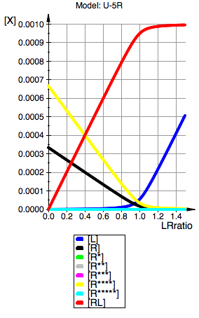
// plot all together
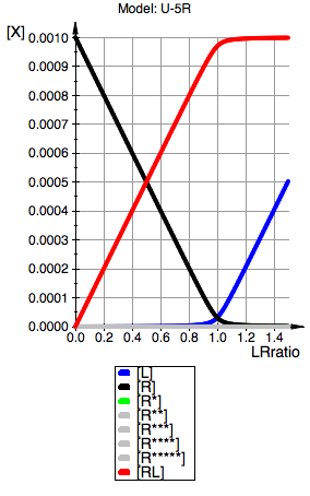
plot(pLeq, pReq, pR_s_1eq, pR_s_2eq, pR_s_3eq, pR_s_4eq, pR_s_5eq, pRLeq,
YAxisTitle="[X]", Header=("Model: ".ProjectName),
Height=160, Width=100,TicksLabelFont=["Helvetica",12,[0,0,0],Left],
AxesTitleFont=["Helvetica",14,[0,0,0],Left],
XGridVisible=TRUE, YGridVisible=TRUE,
LegendVisible=TRUE, LegendFont=["Helvetica",14,[0,0,0],Left],
ViewingBoxYMax=Total_R);
Full model
Model: U-5R
Total_R=0.001
Ka=1000000.0, Kd=0.000001
Kb*=2
Kb**=3
Kb***=4
Kb****=5
Kb*****=6
Kc*-**=3/2
Kc*-***=2
Kc*-****=5/2
Kc*-*****=3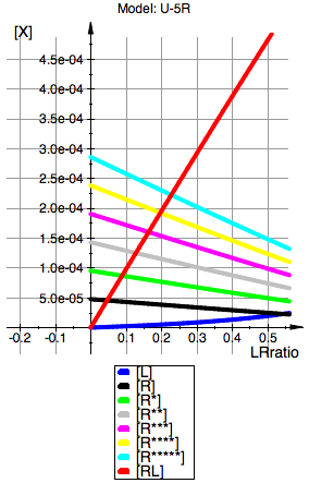
Jump back to the beginning of simulation section
Jump back to the beginning of simulation section
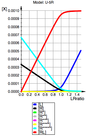
Test of the model: titration of R with L
Full model, then truncated model
|
Reduce to U model |
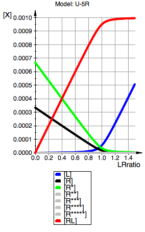
Reduce to U-R (use R*) |
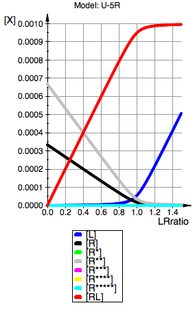
Reduce to U-R (use R**) |
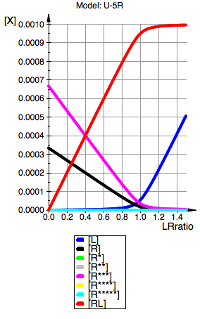
Reduce to U-R (use R***) |
|
Reduce to U-R (use R****) |
Reduce to U-R (use R*****) |
|
|
|
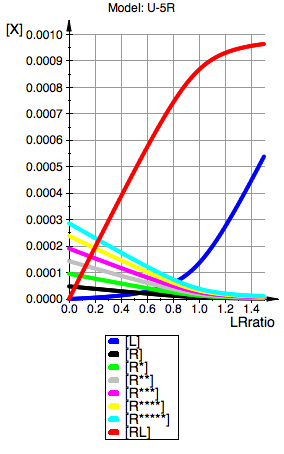
Full model
|
|
|
|
|
|
|
|
|
Conclusion:
The model works as expected