EKM 31
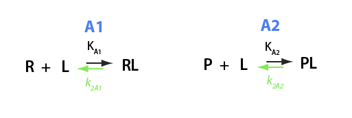
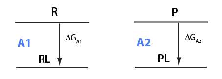
Analysis of the thermodynamic equilibrium relationships for a ligand binding to two different receptors
U__U model
images from /Users/kovrigin/Documents/Workspace/Data/Data.XVIII/EKM31.CON58.Ion_Titrations/1.MuPad_derivations/U__U_model.pdf
Here I will analyze numeric solutions I derived in U__U_derivation.mn for equilibrium between two different receptors competing for the same ligand.
Clean up
reset()
Path to previous results
ProjectName:="U__U";
CurrentPath:="/Users/kovrigin/Documents/Workspace/Data/Data.XVIII/EKM31.CON58.Ion_Titrations/1.MuPad_derivations/"


Read results of derivations
filename:=CurrentPath.ProjectName.".mb";
fread(filename,Quiet):
anames(User)


Assume some values for testing operation
Total_P:=1e-3:
Total_L:=10e-3:
Eq_L:=9e-3:
Ka1:=1e3:
Ka2:=2e4:
Total_R:=0.000006138735421:
test operation of all procedures
pnLeq_U_U(Total_R, Total_P, Total_L, Ka1, Ka2);
pnReq_U_U(Total_R, Total_P, Total_L, Ka1, Ka2);
pnPeq_U_U(Total_R, Total_P, Total_L, Ka1, Ka2);
pnRLeq_U_U(Total_R, Total_P, Total_L, Ka1, Ka2);
pnPLeq_U_U(Total_R, Total_P, Total_L, Ka1, Ka2);

=> OK
Make wrapper functions for plotting
fnLeq:=Total_L -> pnLeq_U_U(Total_R, Total_P, Total_L, Ka1, Ka2):
fnReq:=Total_L -> pnReq_U_U(Total_R, Total_P, Total_L, Ka1, Ka2):
fnPeq:=Total_L -> pnPeq_U_U(Total_R, Total_P, Total_L, Ka1, Ka2):
fnRLeq:=Total_L -> pnRLeq_U_U(Total_R, Total_P, Total_L, Ka1, Ka2):
fnPLeq:=Total_L -> pnPLeq_U_U(Total_R, Total_P, Total_L, Ka1, Ka2):
Test plotting
Total_R:=1e-3:
Total_P:=1e-3:
Total_L_max:=2e-3:
Ka1:=1e3:
Ka2:=1e3:
LineW:=1.5: //line width
// create plots
pLeq:= plot::Function2d(
Function=(fnLeq),
LegendText="[L]",
Color = RGB::Blue,
XMin=(0),
XMax=(Total_L_max),
XName=(L),
TitlePositionX=(0),
LineWidth=LineW):
pRLeq:= plot::Function2d(
Function=(fnRLeq),
LegendText="[RL]",
Color = RGB::Red,
XMin=(0),
XMax=(Total_L_max),
XName=(L),
TitlePositionX=(0),
LineWidth=LineW):
plot(pLeq, pRLeq, LegendVisible=TRUE)
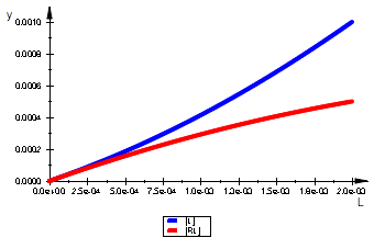
=> OK
Assume some constants and evaluate titrations
Total_R:=1e-3:
Total_P:=1e-3:
Ka1:=1e4:
Ka2:=1e4:
Total_L_max:=2e-3: // plotting range
LineW:=1.5: // plot line width
pLeq:= plot::Function2d(
Function=(fnLeq),
LegendText="[L]",
Color = RGB::Blue,
XMin=(0),
XMax=(Total_L_max),
XName=(L),
TitlePositionX=(0),
LineWidth=LineW):
pReq:= plot::Function2d(
Function=(fnReq),
LegendText="[R]",
Color = RGB::Black,
XMin=(0),
XMax=(Total_L_max),
XName=(L),
TitlePositionX=(0),
LineWidth=LineW):
pPeq:= plot::Function2d(
Function=(fnPeq),
LegendText="[P]",
Color = RGB::Magenta,
XMin=(0),
XMax=(Total_L_max),
XName=(L),
TitlePositionX=(0),
LineWidth=LineW):
pRLeq:= plot::Function2d(
Function=(fnRLeq),
LegendText="[RL]",
Color = RGB::Red,
XMin=(0),
XMax=(Total_L_max),
XName=(L),
TitlePositionX=(0),
LineWidth=LineW):
pPLeq:= plot::Function2d(
Function=(fnPLeq),
LegendText="[PL]",
Color = RGB::Green,
XMin=(0),
XMax=(Total_L_max),
XName=(L),
TitlePositionX=(0),
LineWidth=LineW):
// Text report
print(Unquoted,"Model: ".ProjectName);
print(Unquoted,"Total_R=".Total_R);
print(Unquoted,"Total_P=".Total_P);
Kd1:=1/Ka1:
print(Unquoted,"Ka1=".Ka1." 1/M, Kd1=".Kd1." M");
Kd2:=1/Ka2:
print(Unquoted,"Ka2=".Ka2." 1/M, Kd2=".Kd2." M");
// plot all together
plot(//pLeq,
pReq, pPeq, pRLeq, pPLeq,
YAxisTitle="[X]", Header=("Model: ".ProjectName),
Height=160, Width=100,TicksLabelFont=["Helvetica",12,[0,0,0],Left],
AxesTitleFont=["Helvetica",14,[0,0,0],Left],
XGridVisible=TRUE, YGridVisible=TRUE,
LegendVisible=TRUE, LegendFont=["Helvetica",14,[0,0,0],Left]);
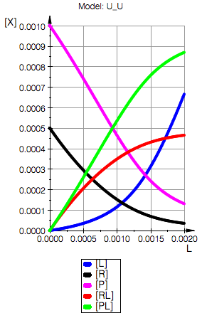
Model: U__U
Total_R=0.001
Total_P=0.001
Ka1=10000.0 1/M, Kd1=0.0001 M
Ka2=10000.0 1/M, Kd2=0.0001 M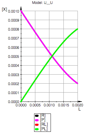
Jump back to the beginning of simulation section
Jump back to the beginning of simulation section
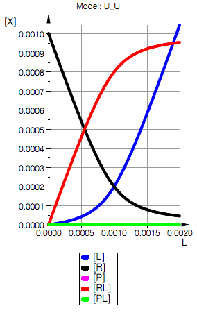
Test of the model: titration of a mixture of P and R with L
|
R only (P not present) |
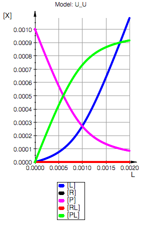
P only (R not present) |
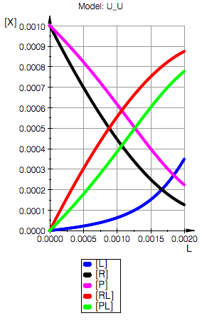
Both P and R present at identical concentrations |
Amount of R is reduced two-fold. |
|
Model: U_U
|
Model: U_U
|
Model: U_U
|
Model: U_U
|
|
Conclusion:
1. Normal saturation curve of RL
|
Conclusion:
1. Normal saturation curve of PL.
2. Addinity of P to L is weaker so we have lower saturation.
|
Conclusion:
1. Overall degree of saturation of RL and PL is smaller than when a competitor is not present.
2. R is binding to L twice as tight. Therefore, degree of saturation of RL is higher than of PL.
3. Ratio between RL and PL is not constant---a consequence of binding reactions being bimolecular and both dependent on concentration of L.
|
Conclusions:
1. Total concentration of binding sites for L is reduced---reflected by higher [L].
2. Total concentration of PL is increased due to reduced competition---fractional saturation of PL is also increased.
3. Fractional saturation of RL is increased at lower concentration of R because of higher ratio of free L to free R For C(L)=0.0012 ---from 65% at 1 mM R to 80% at 0.5 mM R). |
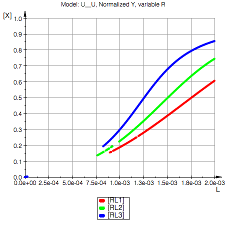
Saturation of R with L at different concentrations of R
print(Unquoted,"Plot a comparative series for fractional saturation of RL at different total concentrations of R (concentration of P is held constant).");
Total_R1:=1.5e-3:
print(Unquoted,"Total_R1=".Total_R1." M");
Total_R2:=1.0e-3:
print(Unquoted,"Total_R2=".Total_R2." M");
Total_R3:=0.5e-3:
print(Unquoted,"Total_R3=".Total_R3." M");
// Other parameters
Total_P:=1e-3:
Ka1:=1e4:
Ka2:=1e5:
print(Unquoted,"Total_P=".Total_P." M");
Kd1:=1/Ka1:
print(Unquoted,"Ka1=".Ka1." 1/M, Kd1=".Kd1." M");
Kd2:=1/Ka2:
print(Unquoted,"Ka2=".Ka2." 1/M, Kd2=".Kd2." M");
// Plot parameters
Total_L_max:=2e-3: // plotting range
LineW:=1.5: // plot line width
print(Unquoted,"Model: ".ProjectName);
// Define normalized functions [RL]/Rtot, [PL]/Ptot and [L]/Ltot
fnRLeqNorm1:=Total_L -> pnRLeq_U_U(Total_R1, Total_P, Total_L, Ka1, Ka2)/Total_R1:
fnRLeqNorm2:=Total_L -> pnRLeq_U_U(Total_R2, Total_P, Total_L, Ka1, Ka2)/Total_R2:
fnRLeqNorm3:=Total_L -> pnRLeq_U_U(Total_R3, Total_P, Total_L, Ka1, Ka2)/Total_R3:
// Generate three plots
pRLeq1:= plot::Function2d(
Function=(fnRLeqNorm1),
LegendText="[RL1]",
Color = RGB::Red,
XMin=(0),
XMax=(Total_L_max),
XName=(L),
TitlePositionX=(0),
LineWidth=LineW):
pRLeq2:= plot::Function2d(
Function=(fnRLeqNorm2),
LegendText="[RL2]",
Color = RGB::Green,
XMin=(0),
XMax=(Total_L_max),
XName=(L),
TitlePositionX=(0),
LineWidth=LineW):
pRLeq3:= plot::Function2d(
Function=(fnRLeqNorm3),
LegendText="[RL3]",
Color = RGB::Blue,
XMin=(0),
XMax=(Total_L_max),
XName=(L),
TitlePositionX=(0),
LineWidth=LineW):
// plot all together
plot(pRLeq1, pRLeq2, pRLeq3,
YAxisTitle="[X]", Header=("Model: ".ProjectName.", Normalized Y, variable R"),
Height=160, Width=160,TicksLabelFont=["Helvetica",12,[0,0,0],Left],
AxesTitleFont=["Helvetica",14,[0,0,0],Left],
XGridVisible=TRUE, YGridVisible=TRUE,
LegendVisible=TRUE, LegendFont=["Helvetica",14,[0,0,0],Left],
ViewingBoxYMax=1);
Plot a comparative series for fractional saturation of RL at different total co\
ncentrations of R (concentration of P is held constant).
Total_R1=0.0015 M
Total_R2=0.001 M
Total_R3=0.0005 M
Total_P=0.001 M
Ka1=10000.0 1/M, Kd1=0.0001 M
Ka2=100000.0 1/M, Kd2=0.00001 M
Model: U__U
Conclusion: Upon reducing total concentration of R we have higher degree of saturaton of R (and P) with L due to reduction in total amount of binding sites in the solution.
Plot a comparative series for fractional saturation of RL at different total co\
ncentrations of R (concentration of P is held constant).
Total_R1=0.0015 M
Total_R2=0.001 M
Total_R3=0.0005 M
Total_P=0.001 M
Ka1=20000.0 1/M, Kd1=0.00005 M
Ka2=10000.0 1/M, Kd2=0.0001 M
Model: U_U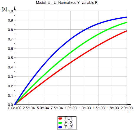
Switched affinities
Plot a comparative series for fractional saturation of RL at different total co\
ncentrations of R (concentration of P is held constant).
Total_R1=0.0015 M
Total_R2=0.001 M
Total_R3=0.0005 M
Total_P=0.001 M
Ka1=10000.0 1/M, Kd1=0.0001 M
Ka2=100000.0 1/M, Kd2=0.00001 M
Model: U__U