U__U_derivation

EKM 31

Derivation of the thermodynamic equilibrium relationships for a ligand binding to two different receptors

U__U model

images from /Users/kovrigin/Documents/Workspace/Data/Data.XVIII/EKM31.CON58.Ion_Titrations/1.MuPad_derivations/U__U_model.pdf

Contents

Goals

1. Definitions

2. Basic equilibrium equations

3. Derivation of equations for equilibrium concentrations

4. Prepare equations for a numeric solution

5. Save results on disk for future use

Conclusions

Back to Contents

Goals

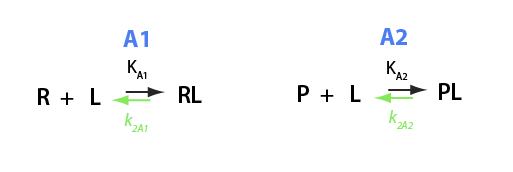
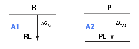
Here I will derive equations for equilibrium between two different receptors competing for the same ligand. Specific case: divalent ion binding to remote site in Ras and, at the same time, to free GNP or EDTA in solution.

Back to Contents

1. Definitions

clean up workspace

reset()

Set path to save results into:

ProjectName:="U__U";
CurrentPath:="/Users/kovrigin/Documents/Workspace/Data/Data.XVIII/EKM31.CON58.Ion_Titrations/1.MuPad_derivations/";

"U__U"
"/Users/kovrigin/Documents/Workspace/Data/Data.XVIII/EKM31.CON58.Ion_Titrations/1.MuPad_derivations/"

Binding and isomerization constants

All binding constants I am using are association constants.

These relationships serve as restraints for solve(), but not restrict these values in calculations!

K_A_1

K_A_1 ;
assumeAlso(K_A_1 > 0):
assumeAlso(K_A_1 , R_)

K_A_1

K_A_2

K_A_2 ;
assumeAlso(K_A_2 > 0):
assumeAlso(K_A_2 , R_):

K_A_2

Total concentrations

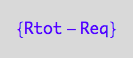
Rtot - total concentration of the receptor

Rtot;
assumeAlso(Rtot>0):
assumeAlso(Rtot,R_):

Rtot

Ltot - total concentration of the first ligand

Ltot;
assumeAlso(Ltot>0):
assumeAlso(Ltot,R_):

Ltot

Ptot - total concentration of the second receptor

Ptot;
assumeAlso(Ptot>0):
assumeAlso(Ptot,R_):

Ptot

Equilibrium concentrations

Req - equilibrium concentration of the first receptor

Req;
assumeAlso(Req>0):
assumeAlso(Req<Rtot):
assumeAlso(Req,R_):

Req

Peq - equilibrium concentration of the second receptor

Peq;
assumeAlso(Peq>0):
assumeAlso(Peq<Ptot):
assumeAlso(Peq,R_):

Peq

Leq - equilibrium concentration of a free ligand

Leq;
assumeAlso(Leq>0):
assumeAlso(Leq<Ltot):
assumeAlso(Leq,R_):

Leq

RLeq - equilibrium concentration of the first receptor-ligand complex

RLeq;
assumeAlso(RLeq>0):
assumeAlso(RLeq<Rtot):
assumeAlso(RLeq,R_):

RLeq

PLeq - equilibrium concentration of the second receptor-ligand complex

PLeq;
assumeAlso(PLeq>0):
assumeAlso(PLeq<Ptot):
assumeAlso(PLeq,R_):

PLeq

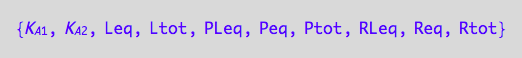
Check what we defined

anames(Properties,User);

${K_A_1, K_A_2, Leq, Ltot, PLeq, Peq, Ptot, RLeq, Req, Rtot}$

Back to Contents

2. Basic equilibrium equations

Mass conservation equations

eq2_1:= Rtot = Req + RLeq;
eq2_2:= Ptot = Peq + PLeq;
eq2_3:= Ltot = Leq + PLeq + RLeq;

Rtot = RLeq + Req
Ptot = PLeq + Peq
Ltot = Leq + PLeq + RLeq

Equilibrium constants

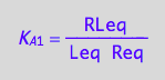
eq2_4:= K_A_1 = RLeq / (Req*Leq);

K_A_1 = RLeq/(Leq*Req)

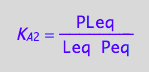
eq2_5:= K_A_2 = PLeq / (Peq*Leq)

K_A_2 = PLeq/(Leq*Peq)

Back to Contents

3. Derivation of equations for equilibrium concentrations

Express Leq as a function of all constants and total concentrations. If insoluble ---express Rtot=f(Leq and all constants).

First, express RLeq and PLeq from mass conservation laws

eq2_1;eq2_2; eq2_3

Rtot = RLeq + Req
Ptot = PLeq + Peq
Ltot = Leq + PLeq + RLeq

RLeq=f(...)

solve(eq2_1,RLeq);
%[1];
eq3_1a:= RLeq = %

{Rtot - Req}

RLeq = Rtot - Req

PLeq=f(...)

solve(eq2_2,PLeq);
%[1];
eq3_1b:= PLeq = %

{Ptot - Peq}

PLeq = Ptot - Peq

Substitute these results into

-> Ltot=f(...)

eq3_1c:= eq2_3 | eq3_1a | eq3_1b

Ltot = Leq - Peq + Ptot - Req + Rtot

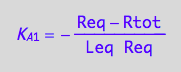
-> K_A_1=f(...)

eq2_4 ;
eq3_3:= % | eq3_1a

K_A_1 = RLeq/(Leq*Req)
K_A_1 = -(Req - Rtot)/(Leq*Req)

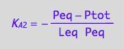
-> K_A_2=f(...)

eq2_5;
eq3_4:= % | eq3_1b

K_A_2 = PLeq/(Leq*Peq)
K_A_2 = -(Peq - Ptot)/(Leq*Peq)

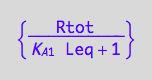
Express Peq and Req from the last equations

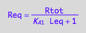
Req=f(...)

eq3_3;
solve(%,Req);
eq3_5:= Req = %[1];

K_A_1 = -(Req - Rtot)/(Leq*Req)
${Rtot/(K_A_1*Leq + 1)}$
Req = Rtot/(K_A_1*Leq + 1)

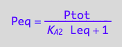
Peq=f(...)

eq3_4;
solve(%,Peq);
eq3_6:= Peq = %[1];

K_A_2 = -(Peq - Ptot)/(Leq*Peq)
${Ptot/(K_A_2*Leq + 1)}$
Peq = Ptot/(K_A_2*Leq + 1)

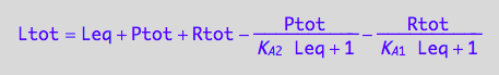
Substitute into mass conservation law for L

Ltot=f(...)

eq3_1c;
% | eq3_5 | eq3_6;
eq3_7:= %:

Ltot = Leq - Peq + Ptot - Req + Rtot
Ltot = Leq + Ptot + Rtot - Ptot/(K_A_2*Leq + 1) - Rtot/(K_A_1*Leq + 1)

Solve it for Leq

solutions3_7:=solve(eq3_7, Leq)

Dom::Interval(0, Ltot) intersect RootOf(K_A_1*K_A_2*X49^3 - K_A_1*K_A_2*Ltot*X49^2 + K_A_1*K_A_2*Ptot*X49^2 + K_A_1*K_A_2*Rtot*X49^2 + K_A_2*X49^2 + K_A_1*X49^2 - K_A_2*Ltot*X49 - K_A_1*Ltot*X49 + K_A_1*Rtot*X49 + K_A_2*Ptot*X49 + X49 - Ltot, X49)

Insoluble.

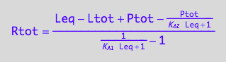
Express Rtot for numeric solution

solve(eq3_7, Rtot):
eq3_8:= Rtot = %[1][1];

Rtot = (Leq - Ltot + Ptot - Ptot/(K_A_2*Leq + 1))/(1/(K_A_1*Leq + 1) - 1)

Back to Contents

4. Prepare equations for a numeric solution

Summary of final equations

ProjectName

"U__U"

Reassign names for storage

Rtot=f([L],...)

Rtot_U_U:=eq3_8

Rtot = (Leq - Ltot + Ptot - Ptot/(K_A_2*Leq + 1))/(1/(K_A_1*Leq + 1) - 1)

[R]=f([L],...)

Req_U_U:=eq3_5

Req = Rtot/(K_A_1*Leq + 1)

[P]=f([L],...)

Peq_U_U:=eq3_6

Peq = Ptot/(K_A_2*Leq + 1)

[RL]=f([L],...)

RLeq_U_U:=eq3_1a

RLeq = Rtot - Req

[PL]=f([L],...)

PLeq_U_U:=eq3_1b

PLeq = Ptot - Peq

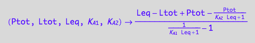
Prepare functions for numeric solution and evaluation

A function for numeric solving for [L].

fRtot_U_U:=(Ptot, Ltot, Leq, K_A_1, K_A_2)--> eq3_8[2]

(Ptot, Ltot, Leq, K_A_1, K_A_2) -> (Leq - Ltot + Ptot - Ptot/(K_A_2*Leq + 1))/(1/(K_A_1*Leq + 1) - 1)

Assume some constant values for testing

Total_P:=1e-3:
Total_L:=10e-3:
Eq_L:=9e-3:
Ka1:=1e3:
Ka2:=2e4:

Test fRtot:

Total_R:=fRtot_U_U(Total_P, Total_L, Eq_L, Ka1, Ka2)

0.000006138735421

=> equation works OK

A procedure for numeric solving of R(tot)=f([L],...) thus creating a function [L]=f(Rtot,...)

WARNING: Make sure the Leq search starts with a non-zero value!

pnLeq_U_U:= proc(Total_R, Total_P, Total_L, Ka1, Ka2)

    /* Parameter names should be different from
      variable names used in the equation!!!

      If you see an error message:
          "Error: Illegal operand [_index];
           during evaluation of 'your function name'"
      it means fsolve returned FAIL and you need to check
      values of all parameters passed to the function fRtot

    */

   local result;
   begin
      // print(Total_R, Total_P, Total_L, Ka1, Ka2);
      // numeric solving equation for Leq in a restricted range.
      // WARNING: make sure the range starts with a non-zero number!!!!
      // Also: variable to solve has to be called 'x' !!!
      result:=numeric::fsolve(
            Total_R-fRtot_U_U(Total_P, Total_L, x, Ka1, Ka2),
            x=10e-32..Total_L);
     // print(result);
     // extract answer from equation
     result[1][2]
end_proc;

`proc pnLeq_U_U(Total_R, Total_P, Total_L, Ka1, Ka2) ... end`

Test its operation

pnLeq_U_U(Total_R, Total_P, Total_L, Ka1, Ka2)

0.009

=> OK

Define procedures to compute equilibrium concentrations of all species

[R]

Req_U_U;
pnReq_U_U:=proc(Total_R, Total_P, Total_L, Ka1, Ka2)
   // Parameter names should be different from
   // variable names used in the equation!!!
   local L;
    begin

      L:=pnLeq_U_U(Total_R, Total_P, Total_L, Ka1, Ka2);

      // Equation for [R]
      Req_U_U[2] | Rtot=Total_R | Leq=L | K_A_1=Ka1;

    end_proc

Req = Rtot/(K_A_1*Leq + 1)
`proc pnReq_U_U(Total_R, Total_P, Total_L, Ka1, Ka2) ... end`

test

pnReq_U_U(Total_R, Total_P, Total_L, Ka1, Ka2);
// test for not having some parameters 'hard-coded' by unwanted substitution.
pnReq_U_U(1, 1, 1, 1, 1);

0.0000006138735421
0.7071067812

=> OK

[P]

Peq_U_U;
pnPeq_U_U:=proc(Total_R, Total_P, Total_L, Ka1, Ka2)
   // Parameter names should be different from
   // variable names used in the equation!!!
   local L;
    begin

      L:=pnLeq_U_U(Total_R, Total_P, Total_L, Ka1, Ka2);

      // Equation for [P]
      Peq_U_U[2] | Ptot=Total_P | Leq=L | K_A_2=Ka2;

    end_proc

Peq = Ptot/(K_A_2*Leq + 1)
`proc pnPeq_U_U(Total_R, Total_P, Total_L, Ka1, Ka2) ... end`

test

pnPeq_U_U(Total_R, Total_P, Total_L, Ka1, Ka2);
// test for not having some parameters 'hard-coded' by unwanted substitution.
pnPeq_U_U(2, 2, 2, 2, 2);

0.000005524861878
1.17539053

[PL]

PLeq_U_U;
pnPLeq_U_U:=proc(Total_R, Total_P, Total_L, Ka1, Ka2)
   // Parameter names should be different from
   // variable names used in the equation!!!
   local L;
    begin

      L:=pnLeq_U_U(Total_R, Total_P, Total_L, Ka1, Ka2);
      P:=pnPeq_U_U(Total_R, Total_P, Total_L, Ka1, Ka2);

      // Equation for [P]
      PLeq_U_U[2] | Ptot=Total_P | Peq=P;

    end_proc

PLeq = Ptot - Peq
`proc pnPLeq_U_U(Total_R, Total_P, Total_L, Ka1, Ka2) ... end`

test

pnPLeq_U_U(Total_R, Total_P, Total_L, Ka1, Ka2);
// test for not having some parameters 'hard-coded' by unwanted substitution.
pnPeq_U_U(2, 2, 2, 2, 2);

0.0009944751381
1.17539053

[RL]

RLeq_U_U;
pnRLeq_U_U:=proc(Total_R, Total_P, Total_L, Ka1, Ka2)
   // Parameter names should be different from
   // variable names used in the equation!!!
   local L;
    begin

      L:=pnLeq_U_U(Total_R, Total_P, Total_L, Ka1, Ka2);
      R:=pnReq_U_U(Total_R, Total_P, Total_L, Ka1, Ka2);

      // Equation for [P]
      RLeq_U_U[2] | Rtot=Total_R | Req=R;

    end_proc

RLeq = Rtot - Req
`proc pnRLeq_U_U(Total_R, Total_P, Total_L, Ka1, Ka2) ... end`

test

pnRLeq_U_U(Total_R, Total_P, Total_L, Ka1, Ka2);
// test for not having some parameters 'hard-coded' by unwanted substitution.
pnReq_U_U(2, 2, 2, 2, 2);

0.000005524861878
1.17539053

Final test of all procedures (use mass conservation laws)

Substitute into mass conservation law equations and observe equalities

eq2_1;
eq2_1 | Rtot=Total_R
| RLeq=pnRLeq_U_U(Total_R, Total_P, Total_L, Ka1, Ka2)
| Req=pnReq_U_U(Total_R, Total_P, Total_L, Ka1, Ka2)

Rtot = RLeq + Req
0.000006138735421 = 0.000006138735421

=>OK

eq2_2;
eq2_2 | Ptot=Total_P
| PLeq=pnPLeq_U_U(Total_R, Total_P, Total_L, Ka1, Ka2)
| Peq=pnPeq_U_U(Total_R, Total_P, Total_L, Ka1, Ka2)

Ptot = PLeq + Peq
0.001 = 0.001

=>OK

eq2_3;
eq2_3 | Ltot=Total_L
      | PLeq=pnPLeq_U_U(Total_R, Total_P, Total_L, Ka1, Ka2)
      | RLeq=pnRLeq_U_U(Total_R, Total_P, Total_L, Ka1, Ka2)
      | Leq=pnLeq_U_U(Total_R, Total_P, Total_L, Ka1, Ka2)

Ltot = Leq + PLeq + RLeq
0.01 = 0.01

=>OK

Back to Contents

5. Save results on disk

(you can retrieve them later by executing: fread(filename,Quiet))

ProjectName

"U__U"

filename:=CurrentPath.ProjectName.".mb";
write(filename,
// Equations
Rtot_U_U,
Req_U_U,
Peq_U_U,
RLeq_U_U,
PLeq_U_U,

// Function for numeric solving
fRtot_U_U,

// Final procedures
pnLeq_U_U,
pnReq_U_U,
pnPeq_U_U,
pnRLeq_U_U,
pnPLeq_U_U)

"/Users/kovrigin/Documents/Workspace/Data/Data.XVIII/EKM31.CON58.Ion_Titrations/1.MuPad_derivations/U__U.mb"

Back to Contents

Conclusions

1. This system is analytically insoluble.

2. I derived numeric solutions and saved them.

Back to Contents