B_macro

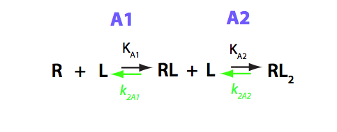
B-macro model: Two L binding to one R molecule

Evgenii Kovrigin, 12/26/2015

Derivation of differential equations describing evolution of spin concentrations

Macroscopic representation (two single-bound species are indistinguishable)

NOTE 1: This is a standard macroscopic model for the receptor binding two ligands to a receptor with two identical sites. I will work out kinetic matrices for both normal labeling scheme (R- NMR active) and try to work with reverse labeling (L- NMR active) as far as I can (EK: did not work out. Results in non-linear equations system).

NOTE 2: The mAcroscopic consideration implicitly adds together concentrations of two single-bound species. This model only applies when both single-bound species have the same chemical shift!

NOTE 3: To utilizing this model together wih microscopic models, which explicitly use concentrations of individual single-bound species, you will need to define a separate model function that formally takes microscopic constants but makes macroscopic ones for input into the B-macro formalism. For statistical effects on thermodynamic and kinetics see

IDAP/Mathematical_models/Equilibrium_thermodynamic_models/B/B_model_derivation.html

Contents

1. Reaction rates and partial conversion rates

3. Net conversion rates

4. Final result for the case when NMR-active nucleus is in R

6. Final result for the reverse labeling: NMR active nucleus is in L

Conclusions

Back to Contents

1. Reaction rates and partial conversion rates

clean up workspace

reset()

We distinguish reaction rates ( Rate, elementary reaction acts per unit time) and conversion rates (dc/dt, number of moles of specific species consumed/produced per unit time). Conversion rates, dc/dt, for species are related to reaction rates, Rate, through molecularity coefficients.

We also distinguish here partial conversion rates from net (overall) conversion rates. The net conversion rate is actual rate of change in measured concentration of the species. Partial conversion rate is the conversion rate of the species along a specific path of the reaction mechanism. By summing all partial conversion rates of the species one obtains the net conversion rate of that species.

Definitions

Equilibrium concentration of R

Req;
assumeAlso(Req > 0); assumeAlso(Req, R_);

Equilibrium concentration of ALL single-bound species, RL

RLeq;
assumeAlso(RLeq > 0); assumeAlso(RLeq, R_);

Equilibrium concentration of RL2

RL2eq;
assumeAlso(RL2eq > 0); assumeAlso(RL2eq, R_);

Equilibrium ligand concentration

Leq;
assumeAlso(Leq > 0); assumeAlso(Leq, R_);

Transition A1 :

R + L = RL

Forward macroscopic rate constant:

k_1_A_1;
assumeAlso(k_1_A_1 >0);
assumeAlso(k_1_A_1, R_);

Reverse macroscopic rate constant:

k_2_A_1;
assumeAlso(k_1_A_1 >0);
assumeAlso(k_1_A_1, R_);

Transition A2:

R + RL = RL2

Macroscopic constants

k_1_A_2;
assumeAlso(k_1_A_2 >0);
assumeAlso(k_1_A_2, R_);

Reverse rate constant

k_2_A_2;
assumeAlso(k_1_A_2 >0);
assumeAlso(k_1_A_2, R_);

Write reaction rates for the properly balanced reactions equations:

Transition A1

1. R + L => LR

a reaction rate

eq1_1a:= Rate_1_A_1 = k_1_A_1*Req*Leq

The partial conversion rate of R (one reaction act USES one molecule of R)

eq1_1b:= dcRdt_1_A_1 = Rate_1_A_1 * (-1)

the final form

eq1_1c:=eq1_1b | eq1_1a

The partial conversion rate of RL (one reaction act MAKES one molecule of RL)

eq1_1d:= dcRLdt_1_A_1 = Rate_1_A_1 * (1)

the final form

eq1_1e:=eq1_1d | eq1_1a

The partial conversion rate of L (one reaction act USES one molecule of L)

eq1_1f:=dcLdt_1_A_1 = Rate_1_A_1 * (-1)

the final form

eq1_1g:= eq1_1f | eq1_1a

2. Ligand dissociation from RL

R + L <= RL

a reaction rate

eq1_2a:= Rate_2_A_1 = k_2_A_1 * RLeq

The partial conversion rate of R (one reaction act MAKES one molecule of R)

eq1_2b:= dcRdt_2_A_1 = Rate_2_A_1 * (1)

the final form

eq1_2c:= eq1_2b | eq1_2a

The partial conversion rate of RL (one reaction act USES one molecule of LaR)

eq1_2d:= dcRLdt_2_A_1 = Rate_2_A_1 * (-1)

the final form

eq1_2e:= eq1_2d | eq1_2a

The partial conversion rate of L (one reaction act MAKES one molecule of L)

eq1_2f:= dcLdt_2_A_1 = Rate_2_A_1 * (1)

the final form

eq1_2g:= eq1_2f | eq1_2a

Transition A2

3. Ligand binding at the second site

RL + L => RL2

a reaction rate

eq1_5a:= Rate_1_A_2 = k_1_A_2 * RLeq * Leq

The partial conversion rate of RL (one reaction act USES one molecule of RL)

eq1_5b:= dcRLdt_1_A_2 = Rate_1_A_2 * (-1)

the final form

eq1_5c:= eq1_5b | eq1_5a

The partial conversion rate of RL2 (one reaction act MAKES one molecule of RL2)

eq1_5d:= dcRL2dt_1_A_2 = Rate_1_A_2 * (1)

the final form

eq1_5e:= eq1_5d | eq1_5a

The partial conversion rate of L (one reaction act USES one molecule of L)

eq1_5f:= dcLdt_1_A_2 = Rate_1_A_2 * (-1)

the final form

eq1_5g:= eq1_5f | eq1_5a

4. Ligand dissociation from RL2

RL + L <= RL2

a reaction rate

eq1_6a:= Rate_2_A_2 = k_2_A_2 * RL2eq

The partial conversion rate of RL2 (one reaction act USES one molecule of RL2)

eq1_6b:= dcRL2dt_2_A_2 = Rate_2_A_2 * (-1)

the final form

eq1_6c:= eq1_6b | eq1_6a

The partial conversion rate of RL (one reaction act MAKES one molecule of RL)

eq1_6d:= dcRLdt_2_A_2 = Rate_2_A_2 * (1)

the final form

eq1_6e:= eq1_6d | eq1_6a

The partial conversion rate of L (one reaction act MAKES one molecule of L)

eq1_6f:= dcLdt_2_A_2 = Rate_2_A_2 * (1)

the final form

eq1_6g:= eq1_6f | eq1_6a

Back to Contents

3. Net conversion rates

To define evolution of the species we need to compute concentrations as a function of time. To this end, we will write differential equations for conversion rates of all species.

In a reversible process both forward and reverse reaction occur simultaneously. Thus, the net conversion rate of the species is a sum of partial conversion rates resulting from forward and reverse reactions along all branches.

Summarize conversion rates and check them against the reaction schematic

A1 transition

eq1_1c; eq1_1e; eq1_1g

eq1_2c; eq1_2e; eq1_2g

A2 transition

eq1_5c; eq1_5e; eq1_5g

eq1_6c; eq1_6e; eq1_6g

=> All seem correct

Net conversion rates

(sum all conversion rates looking at the reaction scheme)

eq3_1a:= dcRdt_N = dcRdt_1_A_1 + dcRdt_2_A_1

eq3_1b:= dcRLdt_N = dcRLdt_1_A_1 + dcRLdt_2_A_1 + dcRLdt_1_A_2 + dcRLdt_2_A_2

RL2

eq3_1c:= dcRL2dt_N = dcRL2dt_1_A_2 + dcRL2dt_2_A_2

eq3_1d:= dcLdt_N = dcLdt_1_A_1 + dcLdt_2_A_1 + dcLdt_1_A_2 + dcLdt_2_A_2

Perform substitutions to obtain net conversion rates expressed in rate constants and concentrations

eq3_1a

list equations for corresponding rates

eq1_1c;eq1_2c;

substitute

eq3_2a:= eq3_1a | eq1_1c | eq1_2c ;

RL (both single-bound species concentrations a lumped together!)

eq3_1b

list equations for corresponding rates

eq1_1e;eq1_2e;eq1_5c;eq1_6e;

substitute

eq3_2b:= eq3_1b | eq1_1e | eq1_2e | eq1_5c | eq1_6e;

RL2

eq3_1c

list equations for corresponding rates

eq1_5e;eq1_6c;

substitute

eq3_2c:= eq3_1c | eq1_5e | eq1_6c ;

eq3_1d

list equations for corresponding rates

eq1_1g;eq1_2g;eq1_5g;eq1_6g;

substitute

eq3_2d:= eq3_1d | eq1_1g | eq1_2g | eq1_5g | eq1_6g;

Back to Contents

4. Final result for NMR-active nucleus included in R

Summarize the derivation results

eq3_2a;eq3_2b;eq3_2c

Assign order to species

eq5_1a:= Req = C1;
eq5_1b:= RLeq = C2;
eq5_1c:= RL2eq = C3;

Assign the same order to the net rates

eq5_2a:= dcRdt_N = dC1dt;
eq5_2b:= dcRLdt_N = dC2dt;
eq5_2c:= dcRL2dt_N = dC3dt;

Restate equations in terms of numbered species

eq5_3a:= eq3_2a | eq5_2a | eq5_2b | eq5_2c | eq5_1a | eq5_1b | eq5_1c

eq5_3b:= eq3_2b | eq5_2a | eq5_2b | eq5_2c | eq5_1a | eq5_1b | eq5_1c

eq5_3c:= eq3_2c | eq5_2a | eq5_2b | eq5_2c | eq5_1a | eq5_1b | eq5_1c

Prepare results for transfer to MATLAB

To avoid typing errors when transfering derived K matrix to MATLAB we type it in here and then directly test against the derivation result from above. After that the K matrix may be transfered to MATLAB by cut-and-paste of the MuPad output.

Enter the K-matrix looking at the above results (collect terms at correspondingly numbered species).

Simple rules that allow catching mistakes in K matrix derivation:

(1) a sum of each column should be zero (so each constant must appear with both positive and negative sign), and

(2) each row has to have complete pairs of constants (i.e., if k12

appears there must be k21 in the same row with an opposite sign and so on).

K_R_NMRactive:=matrix(3,3,[
[ -Leq*k_1_A_1,     k_2_A_1,                       0            ],
[   Leq*k_1_A_1,    -k_2_A_1 - Leq*k_1_A_2,      k_2_A_2         ],
[   0,                         Leq*k_1_A_2,     -k_2_A_2         ]
]);

matrix([[-Leq*k_1_A_1, k_2_A_1, 0], [Leq*k_1_A_1, - k_2_A_1 - Leq*k_1_A_2, k_2_A_2], [0, Leq*k_1_A_2, -k_2_A_2]])

Create a column vector containing concentrations of species in numbered notation

P:=matrix(3,1,[C1,C2,C3])

matrix([[C1], [C2], [C3]])

Check correctness of the entered K matrix by multiplying with P and comparing to the above equations:

Multiply K and P:

dCdt_manual_input:= K_R_NMRactive*P

matrix([[C2*k_2_A_1 - C1*Leq*k_1_A_1], [C3*k_2_A_2 - C2*(k_2_A_1 + Leq*k_1_A_2) + C1*Leq*k_1_A_1], [C2*Leq*k_1_A_2 - C3*k_2_A_2]])

Collect right-hand-side parts of equations (expressions in numbered species)

dCdt_mupad:=matrix(3,1,[ rhs(eq5_3a), rhs(eq5_3b), rhs(eq5_3c)])

matrix([[C2*k_2_A_1 - C1*Leq*k_1_A_1], [C3*k_2_A_2 - C2*k_2_A_1 + C1*Leq*k_1_A_1 - C2*Leq*k_1_A_2], [C2*Leq*k_1_A_2 - C3*k_2_A_2]])

Compare the derivation result to manual input

dCdt_mupad=dCdt_manual_input:
normal(%);
bool(%)

matrix([[C2*k_2_A_1 - C1*Leq*k_1_A_1], [C3*k_2_A_2 - C2*k_2_A_1 + C1*Leq*k_1_A_1 - C2*Leq*k_1_A_2], [C2*Leq*k_1_A_2 - C3*k_2_A_2]]) = matrix([[C2*k_2_A_1 - C1*Leq*k_1_A_1], [C3*k_2_A_2 - C2*k_2_A_1 + C1*Leq*k_1_A_1 - C2*Leq*k_1_A_2], [C2*Leq*k_1_A_2 - C3*k_2_A_2]])

=> If TRUE ---the typed K-matrix is correct.

Use this K-matrix (copy-paste output to MATLAB)

Back to Contents

6. Final result for the "reverse labeling" scheme: the NMR-active nucleus is included in L

The Bloch-McConnell equations describe evolution of bulk magnetization of a sample, which is proportional to the number of spins found in every specific magnetic environment. In case when NMR active nucleus is in L and in the assumption of identical binding sites in this B-macro model, the RL2 contains two spins in the identical environment, therefore the amount of magnetization from spins in the environment of RL2 is proportional to the doubled equilibrium concentration of a dimer.

Summarize the derivation results for L species concentrations

eq3_2b;eq3_2c;eq3_2d;

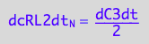
Assign order to species and replace concentrations of molecules with concentrations of spins in them

eq6_1a:= Leq = C1;
eq6_1b:= RLeq = C2;
eq6_1c:= RL2eq = C3/2;

RL2eq = C3/2

Assign the same order to the net rates and replace concentrations of molecules with concentrations of spins in them

eq6_2a:= dcLdt_N = dC1dt;
eq6_2b:= dcRLdt_N = dC2dt;
eq6_2c:= dcRL2dt_N = dC3dt/2;

dcRL2dt_N = dC3dt/2

Restate equations in terms of numbered species

eq3_2d;
eq6_3a:= eq3_2d | eq6_2a | eq6_2b | eq6_2c | eq6_1a | eq6_1b | eq6_1c

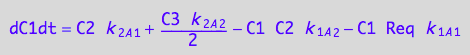
dC1dt = C2*k_2_A_1 + (C3*k_2_A_2)/2 - C1*C2*k_1_A_2 - C1*Req*k_1_A_1

eq3_2b;
eq6_3b:= eq3_2b | eq6_2a | eq6_2b | eq6_2c | eq6_1a | eq6_1b | eq6_1c

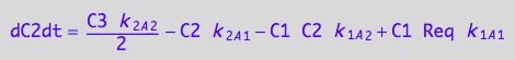
dC2dt = (C3*k_2_A_2)/2 - C2*k_2_A_1 - C1*C2*k_1_A_2 + C1*Req*k_1_A_1

eq3_2c;
eq6_3c:= eq3_2c | eq6_2a | eq6_2b | eq6_2c | eq6_1a | eq6_1b | eq6_1c

dC3dt/2 = C1*C2*k_1_A_2 - (C3*k_2_A_2)/2

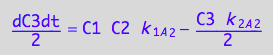
End of story for now. This is not a system of linear equations. It cannot be represented as multiplication of the K matrix and column of populations! To use such a system we need to re-derive the Bloch-McConnell equations using more sophisticated mathematics. Leave it for future...

Back to Contents

Conclusions

I derived differential equations governing spin populations in the "normal" labeling scheme---when NMR-active spin is in the R. The K matrix has been prepared for transferring to MATLAB. The "reverse" labeling scheme produces non-linear system of equations---incompatible with the standard Bloch-McConnell equations and its solution using matrix algebra.

Back to Contents