Testing of the 1D line shape B-macro model (microscopic constants)
Evgenii Kovrigin, 12/27/2015
Contents
- Compute equilibruim populations using B-micro model
- Compute the same populations using microscopic constants in B-macro model
- Create the NMR line shape dataset
- 1. Free receptor
- 2. Saturated receptor
- 3. Equal R:RL:RL2 = 1:2:1
- 4. Dilution of the complex
- 5. Fast exchange in A1 for R:RL:RL2 = 1:2:1
- 6. Fast exchange in A2 for R:RL:RL2 = 1:2:1
Plan
- Set microscopic constants and calculate equilibrium populations using B-micro model with identical sites (parallel paths have the same constant)
- Convert microscopic constants into macroscopic ones the way B_macro_model_1D.m did and use B-macro model to calculate the same populations
- Calculate line shapes with different settings of the rate constants.
close all
clear all
Here you will find all figures
figures_folder='B_macro_testing_figures';
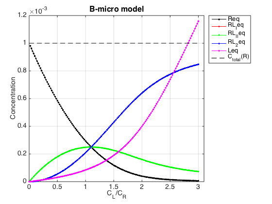
Compute equilibruim populations using B-micro model
NOTE: Use microscopic constants and B-micro model assuming identical sites
Rtotal=1e-3; % Receptor concentration, M
LRratio_array=[0 : 0.02 : 3]; % Array of L/R
K_a_A1_micro=1e4;
K_a_A2_micro=1e4;
% Set parallel paths to identical constants
K_A_1_I = K_a_A1_micro;
K_A_1_I_I = K_a_A1_micro;
K_A_2_I_I = K_a_A2_micro;

% Set appropriate options for the model (see model file for details)
model_numeric_solver='fminbnd'  ;
model_numeric_options=optimset('Diagnostics','off', ...
                    'Display','off',...
                    'TolX',1e-9,...
                    'MaxFunEvals', 1e9);
The important option here is "TolX" that sets termination tolerance on free ligand concentation in molar units. With our solution concentrations in 1e-3 range TolX should be set to some 1e-9.
Compute arrays for populations and plot
concentrations_array=[];
for counter=1:length(LRratio_array)
    % compute
    [concentrations species_names] = equilibrium_thermodynamic_equations.B_micro_model(...
                                                            Rtotal, LRratio_array(counter),...
                                                            K_A_1_I, K_A_1_I_I, K_A_2_I_I,...
                                                            model_numeric_solver, model_numeric_options);
    % collect
    concentrations_array = [concentrations_array ; concentrations];
end
Plot
Figure_title= 'B-micro model';
X_range=[0 max(LRratio_array)+0.1 ]; % extend X just a bit past last point
Y_range=[ ]; % keep automatic scaling for Y
% generate Rtotal array
Rtotal_array = ones(1, length(LRratio_array))*Rtotal;
% display figure
figure_handle=equilibrium_thermodynamic_equations.plot_populations(...
    Rtotal_array, LRratio_array, concentrations_array, species_names, Figure_title, X_range, Y_range);
% save it
results_output.output_figure(figure_handle, figures_folder, 'Concentrations_plot');
Compute the same populations using microscopic constants in B-macro model
Calculate macroscopic constants using the same equations as in B_macro_model_1D.m. Goal: test whether the conversion to macroscopic constants was done correctly
 K_a_A1 = 2*K_a_A1_micro
 K_a_A2 = K_a_A2_micro/2

concentrations_array=[];
for counter=1:length(LRratio_array)
    % compute
    [concentrations species_names] = equilibrium_thermodynamic_equations.B_macro_model(...
        Rtotal, LRratio_array(counter), K_a_A1, K_a_A2,...
        model_numeric_solver, model_numeric_options);
    % collect
    concentrations_array = [concentrations_array ; concentrations];
end
K_a_A1 =
       20000
K_a_A2 =
        5000
Plot
Figure_title= 'B-macro model';
X_range=[0 max(LRratio_array)+0.1 ]; % extend X just a bit past last point
Y_range=[ ]; % keep automatic scaling for Y
% generate Rtotal array
Rtotal_array = ones(1, length(LRratio_array))*Rtotal;
% display figure
figure_handle=equilibrium_thermodynamic_equations.plot_populations(...
    Rtotal_array, LRratio_array, concentrations_array, species_names, Figure_title, X_range, Y_range);
% save it
results_output.output_figure(figure_handle, figures_folder, 'Concentrations_plot');
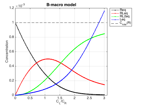
Yes, the conversion to macroscopic constants was correct.
Create the NMR line shape dataset
Create data object for 1D NMR line shapes
test1=NMRLineShapes1D('Simulation','B');
test1.set_active_model('B-macro-model', model_numeric_solver, model_numeric_options)
test1.show_active_model() % to look up necessary parameters of the model
ans =
Active model:
Model 17:  "B-macro-model"
Model description
"1D NMR line shape for the B-macro model with two identical sites using MICROSCOPIC constants, no temperature/field dependence, fminbnd solver"
Model handle: line_shape_equations_1D.B_macro_model_1D
Current solver: fminbnd
Model parameters:
1: Rtotal     2: LRratio     3: log10(K_A1)     4: log10(K_A2)     5: k_2_A1     6: k_2_A2     7: w0_R     8: w0_RL     9: w0_RL2     10: FWHH_R     11: FWHH_RL     12: FWHH_RL2     13: ScaleFactor     14: LRcorrection
Set range for X to extend beyond resonances
w_min= -300;
w_max= 500;
datapoints=100;  % Does not matter much because smooth curve is anyway calculated
test1.set_X(linspace(w_min, w_max, datapoints));
test1.X_range=[w_min w_max]; % this sets display range in the plots
test1.Y_range=[0 18e-5]; % this sets display range in the plots
Calculate ideal data: set noise RMSD to 0 for both X and Y
X_RMSD=0;
Y_RMSD=0;
% *Prepare TotalFit session for easy display of many graphs*
storage_session=TotalFit('All_tests');
1. Free receptor
Use the same thermodynamic parameters as above. Add spectral and kinetic parameters:
LRratio = 0.001 ;
Log10_K_A1 = log10(K_a_A1_micro);
Log10_K_A2 = log10(K_a_A2_micro);
k_2_A1    = 1;   % dissociation rate constant of the complex, 1/s
k_2_A2    = 1;   % dissociation rate constant of the receptor dimer, 1/s
w0_R     = -200;    % NMR frequency of the free receptor R, 1/s
w0_RL    = 200;  % NMR frequency of the dimer R2, 1/s
w0_RL2    = 400;  % NMR frequency of the bound complex RL, 1/s
FWHH_R   = 10;     % line width at half height of the peak of R, 1/s
FWHH_RL  = 10;     % line width at half height of the peak of R2, 1/s
FWHH_RL2  = 10;     % line width at half height of the peak of RL, 1/s
ScaleFactor = 1;  % a multiplier for spectral amplitude (used only when fitting data)
LRcorrection = 1; % default: no correction

% plot line shapes
parameters=[ Rtotal  LRratio   Log10_K_A1   Log10_K_A2  k_2_A1  k_2_A2 ...
     w0_R  w0_RL  w0_RL2  FWHH_R  FWHH_RL  FWHH_RL2  ScaleFactor LRcorrection];


test1.simulate_noisy_data(parameters, X_RMSD, Y_RMSD);
figure_handle=test1.plot_simulation('Free R');
results_output.output_figure(figure_handle, figures_folder, 'Slow_free_R');
% set aside for plotting later
storage_session.copy_dataset_into_array(test1);
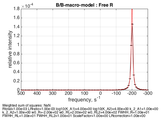
As expected, free receptor signal is centered at w0_R frequency
2. Saturated receptor
% Use the same thermodynamic parameters as above. Add spectral and kinetic parameters:
LRratio = 10 ;
% plot line shapes
parameters=[ Rtotal  LRratio   Log10_K_A1   Log10_K_A2  k_2_A1  k_2_A2 ...
     w0_R  w0_RL  w0_RL2  FWHH_R  FWHH_RL  FWHH_RL2  ScaleFactor LRcorrection];


test1.simulate_noisy_data(parameters, X_RMSD, Y_RMSD);
figure_handle=test1.plot_simulation('Saturated R');
results_output.output_figure(figure_handle, figures_folder, 'Slow_saturated_R');
% set aside for plotting later
storage_session.copy_dataset_into_array(test1);
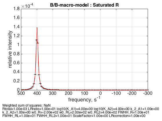
Peak appropriately appears at the w0_RL2 frequency
3. Equal R:RL:RL2 = 1:2:1
LRratio = 1.1;
% plot line shapes
parameters=[ Rtotal  LRratio   Log10_K_A1   Log10_K_A2  k_2_A1  k_2_A2 ...
     w0_R  w0_RL  w0_RL2  FWHH_R  FWHH_RL  FWHH_RL2  ScaleFactor LRcorrection];


test1.simulate_noisy_data(parameters, X_RMSD, Y_RMSD);
figure_handle=test1.plot_simulation('R:RL:RL2 = 1:2:1');
results_output.output_figure(figure_handle, figures_folder, 'middle_point');
% set aside for plotting later
storage_session.copy_dataset_into_array(test1);
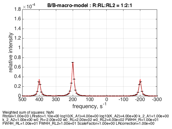
I picked this point because there is exact 1:2:1 ratio between populations at this specific receptor concentration.
4. Dilution of the complex
Rtotal=1e-4;
% plot line shapes
parameters=[ Rtotal  LRratio   Log10_K_A1   Log10_K_A2  k_2_A1  k_2_A2 ...
     w0_R  w0_RL  w0_RL2  FWHH_R  FWHH_RL  FWHH_RL2  ScaleFactor LRcorrection];

test1.Y_range=[0 1e-5]; % this sets display range in the plots

test1.simulate_noisy_data(parameters, X_RMSD, Y_RMSD);
figure_handle=test1.plot_simulation('middle point diluted');
results_output.output_figure(figure_handle, figures_folder, 'middle_point_diluted');
% set aside for plotting later
storage_session.copy_dataset_into_array(test1);
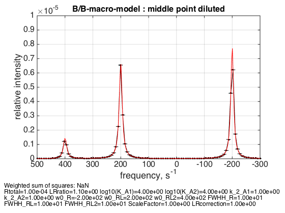
Dilution appropriately shifts equilibrium back.
5. Fast exchange in A1 for R:RL:RL2 = 1:2:1
Rtotal=1e-3;
LRratio = 1.1;
k_2_A1=1000;
k_2_A2=1;

% plot line shapes
parameters=[ Rtotal  LRratio   Log10_K_A1   Log10_K_A2  k_2_A1  k_2_A2 ...
     w0_R  w0_RL  w0_RL2  FWHH_R  FWHH_RL  FWHH_RL2  ScaleFactor LRcorrection];

test1.Y_range=[0 10e-5]; % this sets display range in the plots

test1.simulate_noisy_data(parameters, X_RMSD, Y_RMSD);
figure_handle=test1.plot_simulation('fast A1 at middle point');
results_output.output_figure(figure_handle, figures_folder, 'middle_point_fast_A1');
% set aside for plotting later
storage_session.copy_dataset_into_array(test1);
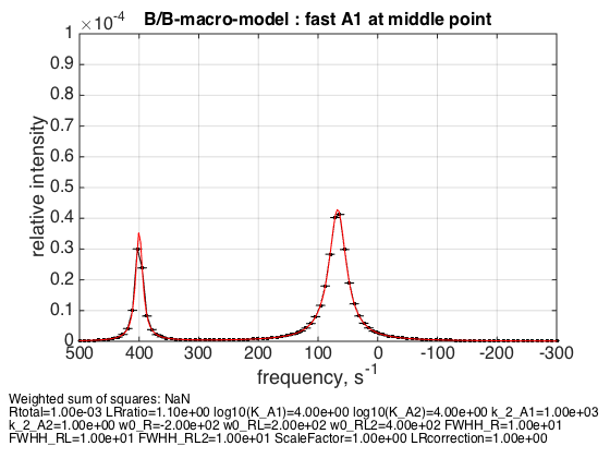
The weighted average peak appears at 1/3 : 2/3 distance between RL and R as expected.
6. Fast exchange in A2 for R:RL:RL2 = 1:2:1
Rtotal=1e-3;
LRratio = 1.1;
k_2_A1=1;
k_2_A2=1000;

% plot line shapes
parameters=[ Rtotal  LRratio   Log10_K_A1   Log10_K_A2  k_2_A1  k_2_A2 ...
     w0_R  w0_RL  w0_RL2  FWHH_R  FWHH_RL  FWHH_RL2  ScaleFactor LRcorrection];

test1.Y_range=[0 10e-5]; % this sets display range in the plots

test1.simulate_noisy_data(parameters, X_RMSD, Y_RMSD);
figure_handle=test1.plot_simulation('fast A2 at middle point');
results_output.output_figure(figure_handle, figures_folder, 'middle_point_fast_A2');
% set aside for plotting later
storage_session.copy_dataset_into_array(test1);
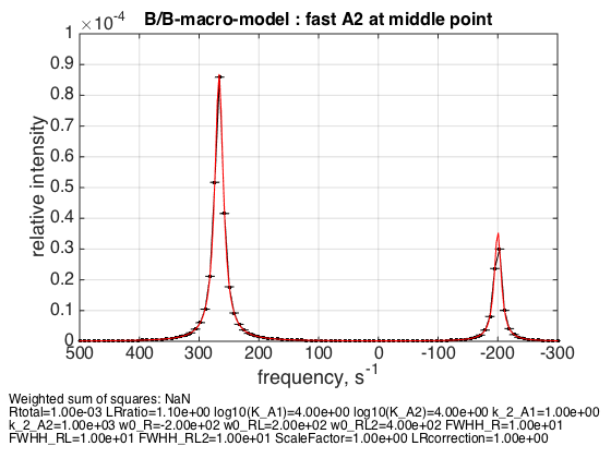
The weighted average peak between RL2 and RL appears at 2/3 : 1/3 distance as expected.
Compare these results to the LineShapeKin Simulation reports with B-micro
IDAP/Mathematical_models/NMR_line_shape_models/1D/B/LineShapeKin_Simulation_reference/Example_simulation
- Tests 1, 2, and 3 : Simulate setup123 slowA1_slowA2
- Tests 3 and 4: Simulate setup34 slowA1_slowA2
- Test 5 : Simulate setup5 fastA1_slowA2
- Test 6 : Simulate setup6 slowA1_fastA2
All tests appeared identical to LineShapeKin Simulation calculations