Derivation of equations for the temperature-dependent I_ab model
Simple intramolecular isomerization; temperature dependence
1. Considerations and Definitions
2. Derivation of a main equation
3. Define functions for equilibrium concentrations
4. Test if solution is meaningful
5. Check whether the solution satisfies all initial equation and conditions
6. Save results on disk for future use
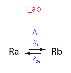
Here, I am introducing temperature dependence into I_ab model.
1. Considerations and Definitions
clean up workspace
reset()
Set path to save results into:
ProjectName:="I_ab_T";
CurrentPath:="/Users/kovrigin/Documents/Workspace/Global Analysis/IDAP/Mathematical_models/NMR_line_shape_models/1D/I_ab_T/";
![]()

Temperature dependent parameters in the model
1. equilibrium constant, K_A;
2. rate constants of forward and reverse transitions, k_1_A and k_2_A;
3. chemical shifts of the species, w_Ra and w_Rb
4. line widths (transverse relaxation rate constants) of the species, FWHH_Ra and FWHH_Rb.
Let's consider them one-by-one.
Equilibrium constant, K_A
The K_A is dependent on temperature via the van't Hoff equation:
eq1_1:= log(K)= -dH/(R*T)+dS/R
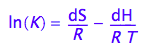
Assumption 1: We will neglect temperature dependence of dH and dS in this treatment (dCp=0)
Rate constants
Assumption 2: We assume that Arrhenius's equation and Eyring's transition state theory are applicable.
The Arrhenius' law connects activation energy, Ea, temperature and the rate constant:
eq1_2:= k=A*exp(-E_a/(R*T))

The activation energy, Ea, is dH of the transition from Ra species to the transition state. The pre-exponential multiplier, A, includes the entropy change of the activation transition and the rate constant for conversion of the transition state into the Rb species, k_t.
eq1_3:= A=k_t*exp(dSa/R)
![]()
Assumption 3: Enthalpy and entropy of activation are not dependent on temperature.
Chemical shifts of the individual species
Chemical shift dependence on temperature may be modelled using empirical linear relationship
eq1_4:= w=a+b*T
![]()
where a and b coefficients are determined from fitting or fixed based on additional assumptions.
Line widths of the individual species
Line widths of the peaks will contain contributions from both the exchange dynamics and overall tumbling of the protein. To accurately fit the exchange contribution we need to estimate the base relaxation rate constant for the specific peak.
Considerations:
1. Base R2 is dependent on the overall tumbling of the molecule through a linear combination of spectral density functions.
2. Spectral density function may be modeled using Lipari-Szabo approach (Cavanaugh et al, 2006, p.368). In this treatment the R2 is roughly a linear function of the rotational correlation time.
eq1_5:= R2=a1+b1*tau_c
![]()
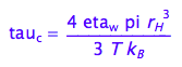
3.The rotational correlation time reduces with temperature according to eq 1.44 (Cavanaugh et al, 2006, p.21)
eq1_6:= tau_c= 4 * pi *eta_w*r_H^3/(3*k_B*T)
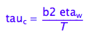
That is of the form:
eq1_7:= tau_c = b2*eta_w/(T)
4. Sovent viscosity in this equation, eta_w, is also inversely temperature-dependent.
// temperature, C, viscosity, microPa*s from CRC Handbook
data:=[
[0, 1793],
[10,1307],
[20, 1002],
[30, 798],
[40, 653]];
p1:=plot::PointList2d(data);
plot(p1);
![]()
![]()
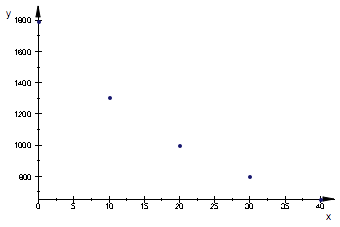
The values for pure water from CRC Handbook, p. 6-2 indicate hyperbolic dependence of the kind
eq1_8:= eta_w= b3/T
![]()
Assumption 4: Changes in viscosity of the NMR sample maybe approximated by changes in pure water viscosity reasonably well.
As a result, the R2 may be approximated by a quadratic hyperbolic function of temperature
eq1_9:= eq1_5 | eq1_7 | eq1_8;
% | a1=a4 | b1=b4/(b2*b3)
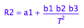
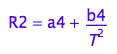
This is the assumed functional dependency of R2 on temperature.
A semi-empirical approach could rely on analysis of linewidths of other resonances from similar protons in the spectrum, which do not undergo conformational exchange. We could fit these peaks with a lorentzian function where FWHH=2*R2 to determine coefficients a4 and b4. By observing large number of peaks we may conclude whether these parameters may be used as global parameters. I expect that b4 will be global parameter while a4 might be individual---reflecting unique R2 of each site.
References
1. Cavanaugh, Fairbrother, Palmer, Rance, Skelton (2006) Protein NMR Spectroscopy: Principles and Practice, Second Edition, Academic Press.
3. CRC Handbook of Chemistry and Physics 87th edition 2006-2007, Ed. Lide DR, Taylor and Francis,
TEMPLATE
Isomerization constant
These relationships serve as restraints for solve(), but not restrict these values in calculations!
K_A
K_A ;
assume(K_A > 0):
assumeAlso(K_A , R_):
![]()
Total concentrations
Rtot - total concentration of the molecule
Rtot;
assumeAlso(Rtot>0):
assumeAlso(Rtot,R_):
![]()
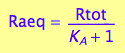
Common equilibrium concentrations
Raeq - equilibrium concentration of Ra form
Raeq;
assumeAlso(Raeq>0):
assumeAlso(Raeq<Rtot):
assumeAlso(Raeq,R_):
![]()
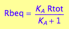
Rbeq - equilibrium concentration of Rb form
Rbeq;
assumeAlso(Rbeq>0):
assumeAlso(Rbeq<Rtot):
assumeAlso(Rbeq,R_):
![]()
anames(Properties,User);
![]()
2. Derivation of a main equation
Total concentrations of the molecule
eq2_1:= Rtot = Raeq + Rbeq
![]()
Write equilibrium thermodynamics equations
eq2_2:= K_A = Rbeq / Raeq

Express Raeq as a function of all constants and total concentrations
Express Rbeq
eq2_2;
solve(%,Rbeq);
%[1][1];
eq2_3:= Rbeq= %

![piecewise([K_A*Raeq in Dom::Interval(0, Rtot), {K_A*Raeq}], [not K_A*Raeq in Dom::Interval(0, Rtot), {}])](I_ab_T_derivation_images/math22.png)
![]()
![]()
Substitute to the mass balance equation
eq2_1;
% | eq2_3;
eq2_4:= %:
![]()
![]()
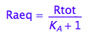
Express Raeq
eq2_4;
solve(%, Raeq);
eq2_5:= Raeq=%[1]
![]()


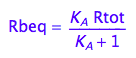
Express Rbeq
eq2_3;
eq2_6:= % | eq2_5;
![]()

Summary of equations for all species
Independent parameters:
Rtot, K_A
![]()
[Ra]
eq2_5
[Rb]
eq2_6
Generate functions
fRaeq:= (Rtot, K_A) --> eq2_5[2]
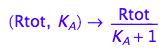
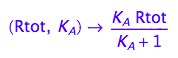
fRbeq:= (Rtot, K_A) --> eq2_6[2]
4. Test if solution is meaningful
Set some realistic values for constants:
Total_R:=1;
Ka:=0.5;
![]()
![]()
Test that all equilibrium concentrations are positive values:
fRaeq(Total_R, Ka);
fRbeq(Total_R, Ka);
if (fRaeq(Total_R, Ka)>0 and
fRbeq(Total_R, Ka)>0
)
then
print(Unquoted,"Solution is meaningful.");
else
print(Unquoted,"WARNING!!!!");
print(Unquoted,"Solution is NOT meaningful: some concentrations become negative!");
end_if
![]()
![]()
Solution is meaningful.
5. Check whether the solution satisfies all initial equation and conditions
Here are all original independent
equations:
eq2_1;eq2_2;
![]()

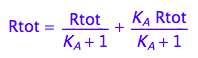
Test eq2_1
eq2_1;
% | eq2_5 | eq2_6;
normal(%);
bool(%)
![]()
![]()
![]()
The found solution satisfies all original equations
5. Save results on disk for future use
(you can retrieve them later by executing: fread(filename,Quiet))
ProjectName
![]()
Eq_Raeq_I_ab:= eq2_5;
Eq_Rbeq_I_ab:= eq2_6;
Reassign function names
fRaeq_I_ab:=fRaeq:
fRbeq_I_ab:=fRbeq:
filename:=CurrentPath.ProjectName.".mb";
write(filename,Eq_Raeq_I_ab,Eq_Rbeq_I_ab, fRaeq_I_ab, fRbeq_I_ab)

Conclusions
1. I derived analytical solutions for the I_ab system