Testing of the U_R2L2 model

by Evgenii Kovrigin, 6/1/2011 A: R+L=RL, B: 2RL=(RL)2

Test Computation of Equilibrium Concentrations
Test of NMR line shape calculations
Create NMR line shape dataset
Free receptor
Slow exchange in B: A fully saturated receptor
Dilution---Slow exchange in B: A fully saturated receptor
Fast exchange in B: A fully saturated receptor
Dilution---Fast exchange in B: A fully saturated receptor
Summary of individual plots
Create a titration series
Conclusions

close all
clear all

Here you will find all figures

figures_folder='U_R2L2_testing_figures';

Test Computation of Equilibrium Concentrations

Set some meaningful parameters

Rtotal=1e-3; % Receptor concentration, M
LRratio_array=[0 : 0.02 : 1.45]; % Array of L/R
K_a_A=1e6;  % Binding affinity constant
K_a_B=1e4;  % Dimerization constant

% Set appropriate options for the model (see model file for details)
model_numeric_solver='fminbnd'  ;

model_numeric_options=optimset('Diagnostics','off', ...
                    'Display','off',...
                    'TolX',1e-9,...
                    'MaxFunEvals', 1e9);

Important option here is TolX that sets termination tolerance on free ligand concentation in molar units. With our solution concentrations in 1e-3 range TolX should be set to some 1e-9.

Compute arrays for populations and plot

concentrations_array=[];
for counter=1:length(LRratio_array)
    % compute
    [concentrations species_names] = equilibrium_thermodynamic_equations.U_R2L2_model(...
        Rtotal, LRratio_array(counter), K_a_A, K_a_B,...
        model_numeric_solver, model_numeric_options);
    % collect
    concentrations_array = [concentrations_array ; concentrations];
end

Plot

Figure_title= 'U-R2L2 model';
X_range=[0 max(LRratio_array)+0.1 ]; % extend X just a bit past last point
Y_range=[ ]; % keep automatic scaling for Y
% display figure
figure_handle=equilibrium_thermodynamic_equations.plot_populations(...
    LRratio_array, concentrations_array, species_names, Figure_title, X_range, Y_range);
% save it
results_output.output_figure(figure_handle, figures_folder, 'Concentrations_plot');

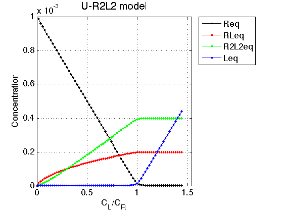
Observations The result is exactly what we expect from this model.

As ligand is added, the ligand-receptor complex is formed. The ratio between the two forms, RL and (RL)2 changes in favor of a dimer as the bound species accumulate. NOTE: A dimer contains two monomers so concentration of spins in line shape calculations will be twice as large for dimers!

Conclusion

The model equilibrium_thermodynamic_equations.U_R2L2_model() works well.

Test of NMR line shape calculations

We will generate line shapes in conditions where we can expect specific patterns. We will plot a spectrum at a specific solution conditions (we will not use Series of datasets for simplicity).

1. Ligand-free receptor should give one peak 2. Saturated receptor, slow exchange between the monomer and a dimer---two distinct peaks for RL and R2L2 species. 3. Saturated receptor, fast exchange - weighted average peak 4. Dilution of saturated receptor---redistribution of peak areas in slow exchange case towards a monomer, and a peak shift in fast exchange case towards a monomer.

Create NMR line shape dataset

Create data object for 1D NMR line shapes

test1=NMRLineShapes1D('Simulation','U-R2L2 test');
test1.set_active_model('U_R2L2-model', model_numeric_solver, model_numeric_options)
test1.show_active_model() % to look up necessary parameters of the model

ans =

Active model:
Model 11:  "U_R2L2-model"
Model description
"1D NMR line shape for the U-R2L2 model, no temperature/field dependence, analytical"
Model handle: line_shape_equations_1D.U_R2L2_model_1D
Current solver: fminbnd
Model parameters: 
1: Rtotal     2: LRratio     3: log10(K_A)     4: log10(K_B)     5: k_2_A     6: k_2_B     7: w0_R     8: w0_RL     9: w0_R2L2     10: FWHH_R     11: FWHH_RL     12: FWHH_R2L2     13: ScaleFactor

Set range for X to extend beyond resonances

w_min= -300;
w_max= 500;
datapoints=100;  % Does not matter much because smooth curve is anyway calculated
test1.set_X(linspace(w_min, w_max, datapoints));

Set fixed plotting ranges for easier comparison If we do not set ranges they will be chosen automatically for each graph

test1.X_range=[w_min w_max]; % this sets display range in the plots
test1.Y_range=[0 8e-5]; % this sets display range in the plots

Calculate ideal data: set noise RMSD to 0 for both X and Y

X_RMSD=0;
Y_RMSD=0;

Free receptor

Use the same thermodynamic parameters as above. Add spectral and kinetic parameters:

LRratio = 0.01 ;  % NOTE: this value cannot be too small! Solution becomes unstable.
Log10_K_A = log10(K_a_A);
Log10_K_B = log10(K_a_B);
k_2_A    = 1;   % dissociation rate constant of the complex, 1/s
k_2_B    = 1;   % dissociation rate constant of the receptor dimer, 1/s
w0_R     = -200;    % NMR frequency of the free receptor R, 1/s
w0_RL    = 200;  % NMR frequency of the dimer R2, 1/s
w0_R2L2    = 400;  % NMR frequency of the bound complex RL, 1/s
FWHH_R   = 20;     % line width at half height of the peak of R, 1/s
FWHH_RL  = 20;     % line width at half height of the peak of R2, 1/s
FWHH_R2L2  = 20;     % line width at half height of the peak of RL, 1/s
ScaleFactor = 1;  % a multiplier for spectral amplitude (used only when fitting data)

% compute equilbrium concentrations
[concentrations species_names] = equilibrium_thermodynamic_equations.U_R2L2_model(...
        Rtotal, LRratio, K_a_A, K_a_B,...
        model_numeric_solver, model_numeric_options)


% plot line shapes
parameters=[ Rtotal  LRratio   Log10_K_A   Log10_K_B  k_2_A  k_2_B ...
     w0_R  w0_RL  w0_R2L2  FWHH_R  FWHH_RL  FWHH_R2L2  ScaleFactor ];


test1.simulate_noisy_data(parameters, X_RMSD, Y_RMSD);
figure_handle=test1.plot_simulation('Slow: free R');
results_output.output_figure(figure_handle, figures_folder, 'Slow_concentrated_R');

concentrations =

   1.0e-03 *

    0.9614    0.0085    0.0007    0.0000


species_names = 

    'Req'    'RLeq'    'R2L2eq'    'Leq'

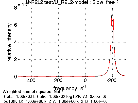
Expected R peak.

Prepare TotalFit session for easy display of many graphs

storage_session=TotalFit('All_tests');
% set aside for plotting later
storage_session.copy_dataset_into_array(test1);

Slow exchange in B: A fully saturated receptor

LRratio = 10 ;
parameters=[ Rtotal  LRratio   Log10_K_A   Log10_K_B  k_2_A  k_2_B ...
     w0_R  w0_RL  w0_R2L2  FWHH_R  FWHH_RL  FWHH_R2L2  ScaleFactor ];

test1.simulate_noisy_data(parameters, X_RMSD, Y_RMSD);
figure_handle=test1.plot_simulation('saturated RL');
results_output.output_figure(figure_handle, figures_folder, 'Saturated_RL');
% set aside for plotting later
storage_session.copy_dataset_into_array(test1);

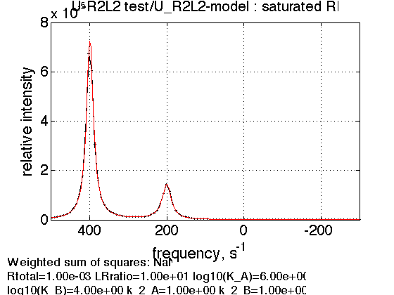
We observe a peaks at frequencies of monomeric and dimeric bound forms with 1:4 ratio of areas (corresponding to 1:2 ratio of molar concentrations of RL and R2L2).

Dilution---Slow exchange in B: A fully saturated receptor

Rtotal = 1e-4 ;
% compute equilbrium concentrations
[concentrations species_names] = equilibrium_thermodynamic_equations.U_R2L2_model(...
        Rtotal, LRratio, K_a_A, K_a_B,...
        model_numeric_solver, model_numeric_options)

parameters=[ Rtotal  LRratio   Log10_K_A   Log10_K_B  k_2_A  k_2_B ...
     w0_R  w0_RL  w0_R2L2  FWHH_R  FWHH_RL  FWHH_R2L2  ScaleFactor ];

test1.simulate_noisy_data(parameters, X_RMSD, Y_RMSD);
figure_handle=test1.plot_simulation('diluted saturated RL');
results_output.output_figure(figure_handle, figures_folder, 'Diluted_Saturated_RL');
% set aside for plotting later
storage_session.copy_dataset_into_array(test1);

concentrations =

   1.0e-03 *

    0.0001    0.0500    0.0250    0.9001


species_names = 

    'Req'    'RLeq'    'R2L2eq'    'Leq'

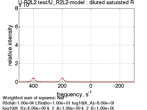
We observe a peaks at frequencies of monomeric and dimeric bound forms with 1:1 ratio of areas (corresponding to 1:0.5 ratio of molar concentrations of RL and R2L2 at reduced total concentration).

Fast exchange in B: A fully saturated receptor

Rtotal = 1e-3 ;
k_2_B=1000;

parameters=[ Rtotal  LRratio   Log10_K_A   Log10_K_B  k_2_A  k_2_B ...
    w0_R  w0_RL  w0_R2L2  FWHH_R  FWHH_RL  FWHH_R2L2  ScaleFactor ];

test1.simulate_noisy_data(parameters, X_RMSD, Y_RMSD);
figure_handle=test1.plot_simulation('FastEx saturated RL');
results_output.output_figure(figure_handle, figures_folder, 'FastEx_Saturated_RL');
% set aside for plotting later
storage_session.copy_dataset_into_array(test1);

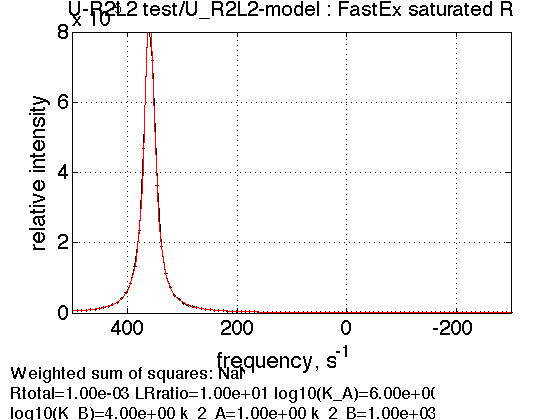
We observe a weighted average peak of monomeric and dimeric bound forms positioned between the two frequencies corresponding to 1:4 spin population ratio.

Dilution---Fast exchange in B: A fully saturated receptor

Rtotal = 1e-4 ;

parameters=[ Rtotal  LRratio   Log10_K_A   Log10_K_B  k_2_A  k_2_B ...
     w0_R  w0_RL  w0_R2L2  FWHH_R  FWHH_RL  FWHH_R2L2  ScaleFactor ];

test1.simulate_noisy_data(parameters, X_RMSD, Y_RMSD);
figure_handle=test1.plot_simulation('Diluted FastEx saturated RL');
results_output.output_figure(figure_handle, figures_folder, 'Diluted_FastEx_Saturated_RL');
% set aside for plotting later
storage_session.copy_dataset_into_array(test1);

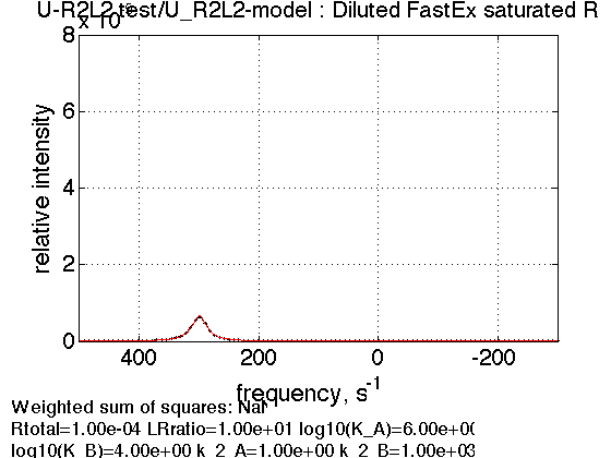
Fast exchange peak now is in the middle corresponding to 1:0.5 ratio of molar concentrations of RL and R2L2 and 1:1 spin populations.

Summary of individual plots

storage_session.define_series('All-tests',1:length(storage_session.dataset_array));
figure_handle=storage_session.plot_1D_series('All-tests', 'All tests', 0);
results_output.output_figure(figure_handle, figures_folder, 'All_tests');

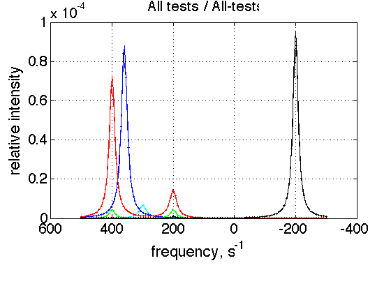
This is a comparison graph of all previous plots

Create a titration series

(see Tutorial 3 for details) Choose parameters

ZERO_LRratio= 0.01; % This number cannot be too small---the model is numeric and will NOT converge!
LRratio_vector=[ZERO_LRratio  0.2   0.4   0.6  0.8   1.0   1.2   1.4 ];


% choose the same parameters as above
session_name='Series';
session=TotalFit(session_name);
series_name='U-R2L2_simulation';
dataset_class_name='NMRLineShapes1D';
model_name='U_R2L2-model';
number_of_datasets=length(LRratio_vector);
X_column=test1.X; % use the same range

% create TotalFit session
session.create_simulation_series(series_name, dataset_class_name, model_name, ...
                 model_numeric_solver, model_numeric_options,...
                 number_of_datasets, X_column);

session.initialize_relation_matrix(sprintf('%s.all_datasets.txt', session_name));

% link parameters
parameter_number_array=[ 1    3 4 5 6 7 8 9 10 11 12 13];
session.batch_link_parameters_in_series(series_name, parameter_number_array);
session.generate_fitting_environment(sprintf('%s.fitting_environment.txt', session_name))

% prepare parameters
first_dataset_index=session.dataset_index(series_name,1);
FAKE_VALUE=1E-6;  % individual (unlinked) parameters: to be assigned later

ideal_parameters=[ Rtotal  FAKE_VALUE   Log10_K_A   Log10_K_B  k_2_A  k_2_B ...
     w0_R  w0_RL  w0_R2L2  FWHH_R  FWHH_RL  FWHH_R2L2  ScaleFactor  ];

% prepare formal limits
fake_limits=zeros(1,length(ideal_parameters));
Monte_Carlo_range_min=fake_limits;
Monte_Carlo_range_max=fake_limits;
parameter_limits_min=fake_limits;
parameter_limits_max=fake_limits;

% assign
session.assign_parameter_values(first_dataset_index, ideal_parameters, ...
        Monte_Carlo_range_min, Monte_Carlo_range_max, parameter_limits_min, parameter_limits_max);

% Assign unlinked LRratio and ranges
parameter_number=2;
values_array=LRratio_vector;

unlinked_fake_ranges=zeros(1,number_of_datasets);
MonteCarlo_range_min_array=unlinked_fake_ranges;
MonteCarlo_range_max_array=unlinked_fake_ranges;
parameter_limits_min_array=unlinked_fake_ranges;
parameter_limits_max_array=unlinked_fake_ranges;

session.assign_unlinked_parameter_in_series(...
             series_name, parameter_number, values_array, ...
             MonteCarlo_range_min_array, MonteCarlo_range_max_array, ...
             parameter_limits_min_array, parameter_limits_max_array);

% Simulate series
X_standard_dev=0;
Y_standard_dev=1e-8;  % something really small
session.simulate_series(series_name, X_standard_dev, Y_standard_dev);

% Plot
Y_offset_percent=10;  % to offset figures vertically for easier viewing
% set plotting ranges
X_range=test1.X_range;  % use old
Y_range=[];  % automatic
session.set_XY_ranges_series(series_name, X_range, Y_range)
figure_handle=session.plot_1D_series(series_name, session.name, Y_offset_percent);
results_output.output_figure(figure_handle, figures_folder, 'Series');

Dataset listing is written to "Series.all_datasets.txt".

Fitting environment saved in Series.fitting_environment.txt.

ans =

New parameter relations (indexed as in all_parameters vector):

[1]     1:Rtotal | 2:Rtotal | 3:Rtotal | 4:Rtotal | 5:Rtotal | 6:Rtotal | 7:Rtotal | 8:Rtotal
[2]     1:LRratio
[3]     1:log10(K_A) | 2:log10(K_A) | 3:log10(K_A) | 4:log10(K_A) | 5:log10(K_A) | 6:log10(K_A) | 7:log10(K_A) | 8:log10(K_A)
[4]     1:log10(K_B) | 2:log10(K_B) | 3:log10(K_B) | 4:log10(K_B) | 5:log10(K_B) | 6:log10(K_B) | 7:log10(K_B) | 8:log10(K_B)
[5]     1:k_2_A | 2:k_2_A | 3:k_2_A | 4:k_2_A | 5:k_2_A | 6:k_2_A | 7:k_2_A | 8:k_2_A
[6]     1:k_2_B | 2:k_2_B | 3:k_2_B | 4:k_2_B | 5:k_2_B | 6:k_2_B | 7:k_2_B | 8:k_2_B
[7]     1:w0_R | 2:w0_R | 3:w0_R | 4:w0_R | 5:w0_R | 6:w0_R | 7:w0_R | 8:w0_R
[8]     1:w0_RL | 2:w0_RL | 3:w0_RL | 4:w0_RL | 5:w0_RL | 6:w0_RL | 7:w0_RL | 8:w0_RL
[9]     1:w0_R2L2 | 2:w0_R2L2 | 3:w0_R2L2 | 4:w0_R2L2 | 5:w0_R2L2 | 6:w0_R2L2 | 7:w0_R2L2 | 8:w0_R2L2
[10]     1:FWHH_R | 2:FWHH_R | 3:FWHH_R | 4:FWHH_R | 5:FWHH_R | 6:FWHH_R | 7:FWHH_R | 8:FWHH_R
[11]     1:FWHH_RL | 2:FWHH_RL | 3:FWHH_RL | 4:FWHH_RL | 5:FWHH_RL | 6:FWHH_RL | 7:FWHH_RL | 8:FWHH_RL
[12]     1:FWHH_R2L2 | 2:FWHH_R2L2 | 3:FWHH_R2L2 | 4:FWHH_R2L2 | 5:FWHH_R2L2 | 6:FWHH_R2L2 | 7:FWHH_R2L2 | 8:FWHH_R2L2
[13]     1:ScaleFactor | 2:ScaleFactor | 3:ScaleFactor | 4:ScaleFactor | 5:ScaleFactor | 6:ScaleFactor | 7:ScaleFactor | 8:ScaleFactor
[14]   n/a
[15]     2:LRratio
[16]   n/a
[17]   n/a
[18]   n/a
[19]   n/a
[20]   n/a
[21]   n/a
[22]   n/a
[23]   n/a
[24]   n/a
[25]   n/a
[26]   n/a
[27]   n/a
[28]     3:LRratio
[29]   n/a
[30]   n/a
[31]   n/a
[32]   n/a
[33]   n/a
[34]   n/a
[35]   n/a
[36]   n/a
[37]   n/a
[38]   n/a
[39]   n/a
[40]   n/a
[41]     4:LRratio
[42]   n/a
[43]   n/a
[44]   n/a
[45]   n/a
[46]   n/a
[47]   n/a
[48]   n/a
[49]   n/a
[50]   n/a
[51]   n/a
[52]   n/a
[53]   n/a
[54]     5:LRratio
[55]   n/a
[56]   n/a
[57]   n/a
[58]   n/a
[59]   n/a
[60]   n/a
[61]   n/a
[62]   n/a
[63]   n/a
[64]   n/a
[65]   n/a
[66]   n/a
[67]     6:LRratio
[68]   n/a
[69]   n/a
[70]   n/a
[71]   n/a
[72]   n/a
[73]   n/a
[74]   n/a
[75]   n/a
[76]   n/a
[77]   n/a
[78]   n/a
[79]   n/a
[80]     7:LRratio
[81]   n/a
[82]   n/a
[83]   n/a
[84]   n/a
[85]   n/a
[86]   n/a
[87]   n/a
[88]   n/a
[89]   n/a
[90]   n/a
[91]   n/a
[92]   n/a
[93]     8:LRratio
[94]   n/a
[95]   n/a
[96]   n/a
[97]   n/a
[98]   n/a
[99]   n/a
[100]   n/a
[101]   n/a
[102]   n/a
[103]   n/a
[104]   n/a

Summary of datasets with lookup vectors (position of each parameter in all_parameter vector)
--------
Dataset 1/U-R2L2_simulation-1,  model "U_R2L2-model"
Parameters          :    Rtotal    LRratio    log10(K_A)    log10(K_B)    k_2_A    k_2_B    w0_R    w0_RL    w0_R2L2    FWHH_R    FWHH_RL    FWHH_R2L2    ScaleFactor
Lookup vector       :   1   2   3   4   5   6   7   8   9   10   11   12   13

Dataset 2/U-R2L2_simulation-2,  model "U_R2L2-model"
Parameters          :    Rtotal    LRratio    log10(K_A)    log10(K_B)    k_2_A    k_2_B    w0_R    w0_RL    w0_R2L2    FWHH_R    FWHH_RL    FWHH_R2L2    ScaleFactor
Lookup vector       :   1   15   3   4   5   6   7   8   9   10   11   12   13

Dataset 3/U-R2L2_simulation-3,  model "U_R2L2-model"
Parameters          :    Rtotal    LRratio    log10(K_A)    log10(K_B)    k_2_A    k_2_B    w0_R    w0_RL    w0_R2L2    FWHH_R    FWHH_RL    FWHH_R2L2    ScaleFactor
Lookup vector       :   1   28   3   4   5   6   7   8   9   10   11   12   13

Dataset 4/U-R2L2_simulation-4,  model "U_R2L2-model"
Parameters          :    Rtotal    LRratio    log10(K_A)    log10(K_B)    k_2_A    k_2_B    w0_R    w0_RL    w0_R2L2    FWHH_R    FWHH_RL    FWHH_R2L2    ScaleFactor
Lookup vector       :   1   41   3   4   5   6   7   8   9   10   11   12   13

Dataset 5/U-R2L2_simulation-5,  model "U_R2L2-model"
Parameters          :    Rtotal    LRratio    log10(K_A)    log10(K_B)    k_2_A    k_2_B    w0_R    w0_RL    w0_R2L2    FWHH_R    FWHH_RL    FWHH_R2L2    ScaleFactor
Lookup vector       :   1   54   3   4   5   6   7   8   9   10   11   12   13

Dataset 6/U-R2L2_simulation-6,  model "U_R2L2-model"
Parameters          :    Rtotal    LRratio    log10(K_A)    log10(K_B)    k_2_A    k_2_B    w0_R    w0_RL    w0_R2L2    FWHH_R    FWHH_RL    FWHH_R2L2    ScaleFactor
Lookup vector       :   1   67   3   4   5   6   7   8   9   10   11   12   13

Dataset 7/U-R2L2_simulation-7,  model "U_R2L2-model"
Parameters          :    Rtotal    LRratio    log10(K_A)    log10(K_B)    k_2_A    k_2_B    w0_R    w0_RL    w0_R2L2    FWHH_R    FWHH_RL    FWHH_R2L2    ScaleFactor
Lookup vector       :   1   80   3   4   5   6   7   8   9   10   11   12   13

Dataset 8/U-R2L2_simulation-8,  model "U_R2L2-model"
Parameters          :    Rtotal    LRratio    log10(K_A)    log10(K_B)    k_2_A    k_2_B    w0_R    w0_RL    w0_R2L2    FWHH_R    FWHH_RL    FWHH_R2L2    ScaleFactor
Lookup vector       :   1   93   3   4   5   6   7   8   9   10   11   12   13

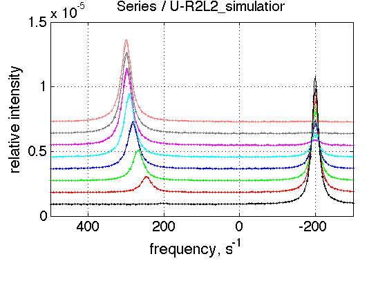
This is an expected result. Binding in slow exchange leads to appearance of a separate resonance, which is a fast-exchange weighted average between RL and (RL)2. As the titration progresses, concentration of a bound complex increases, which shifts dimerization equilbirium towards the dimer. Since we set dimerization to be in fast exchange---we observe a peak shift of a "bound" resonance upon titration progress.

Conclusions

The U-R2L2 model for NMR 1D line shapes works as expected.