Testing of the U_RL model
Evgenii Kovrigin, 6/1/2011
Contents
- TEST COMPUTATION OF EQUILIBRIUM POPULATIONS
- TEST OF NMR LINE SHAPE CALCULATION
- Create NMR line shape dataset
- 1. Free receptor
- 2. Saturated receptor
- 3. Dilution of the complex
- 4. Fast exchange in the complex
- 5. Fast exchange in the diluted complex
- Summary of individual plots
- Create a titration series
- CONCLUSIONS
close all
clear all
Here you will find all figures
figures_folder='U_RL_testing_figures';
TEST COMPUTATION OF EQUILIBRIUM POPULATIONS
Set some meaningful parameters
Rtotal=1e-3; % Receptor concentration, M
LRratio_array=[0 : 0.02 : 1.45]; % Array of L/R
K_a_A=1e6;  % Binding affinity constant
K_a_B=4;  % Isomerization constant

% Set appropriate options for the model (see model file for details)
model_numeric_solver='analytical'  ;

model_numeric_options='none';
Important option here is TolX that sets termination tolerance on free ligand concentation in molar units. With our solution concentrations in 1e-3 range TolX should be set to some 1e-9.
Compute arrays for populations and plot
concentrations_array=[];
for counter=1:length(LRratio_array)
    % compute
    [concentrations species_names] = equilibrium_thermodynamic_equations.U_RL_model(...
        Rtotal, LRratio_array(counter), K_a_A, K_a_B,...
        model_numeric_solver, model_numeric_options);
    % collect
    concentrations_array = [concentrations_array ; concentrations];
end
Plot
Figure_title= 'U-RL model';
X_range=[0 max(LRratio_array)+0.1 ]; % extend X just a bit past last point
Y_range=[ ]; % keep automatic scaling for Y
% display figure
figure_handle=equilibrium_thermodynamic_equations.plot_populations(...
    LRratio_array, concentrations_array, species_names, Figure_title, X_range, Y_range);
% save it
results_output.output_figure(figure_handle, figures_folder, 'Concentrations_plot');
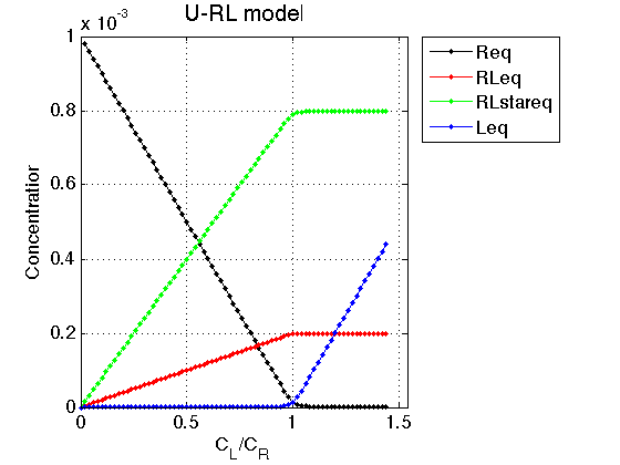
Observations The result is exactly what we expect from this model.
As ligand is added, the ligand-receptor complex is formed species is formed at a constant ratio between the two forms, RL and RL*
Conclusion
The model equilibrium_thermodynamic_equations.U_RL_model() works well.
TEST OF NMR LINE SHAPE CALCULATION
We will generate line shapes in conditions where we can expect specific patterns. We will plot a spectrum at a specific solution conditions
1. Ligand-free receptor in slow exchange should show one peak
2. Saturated receptor should have two peaks in slow exchange. Ratio between peak areas should be independent of Rtotal
3. Fast exchange in the same conditions should yield one averaged peak.
Create NMR line shape dataset
Create data object for 1D NMR line shapes
test1=NMRLineShapes1D('Simulation','U-R test');
test1.set_active_model('U_RL-model', model_numeric_solver, model_numeric_options)
test1.show_active_model() % to look up necessary parameters of the model
ans =

Active model:
Model 8:  "U_RL-model"
Model description
"1D NMR line shape for the U-RL model, no temperature/field dependence, analytical"
Model handle: line_shape_equations_1D.U_RL_model_1D
Current solver: analytical
Model parameters:
1: Rtotal     2: LRratio     3: log10(K_A)     4: log10(K_B)     5: k_2_A     6: k_2_B     7: w0_R     8: w0_RL     9: w0_RLstar     10: FWHH_R     11: FWHH_RL     12: FWHH_RLstar     13: ScaleFactor
Set range for X to extend beyond resonances
w_min= -300;
w_max= 500;
datapoints=100;  % Does not matter much because smooth curve is anyway calculated
test1.set_X(linspace(w_min, w_max, datapoints));
test1.X_range=[w_min w_max]; % this sets display range in the plots
test1.Y_range=[0 8e-5]; % this sets display range in the plots
Calculate ideal data: set noise RMSD to 0 for both X and Y
X_RMSD=0;
Y_RMSD=0;
1. Free receptor
Use the same thermodynamic parameters as above. Add spectral and kinetic parameters:
LRratio = 0.001 ;
Log10_K_A = log10(K_a_A);
Log10_K_B = log10(K_a_B);
k_2_A    = 1;   % dissociation rate constant of the complex, 1/s
k_2_B    = 1;   % dissociation rate constant of the receptor dimer, 1/s
w0_R     = -200;    % NMR frequency of the free receptor R, 1/s
w0_RL    = 200;  % NMR frequency of the dimer R2, 1/s
w0_RLstar    = 400;  % NMR frequency of the bound complex RL, 1/s
FWHH_R   = 10;     % line width at half height of the peak of R, 1/s
FWHH_RL  = 10;     % line width at half height of the peak of R2, 1/s
FWHH_RLstar  = 10;     % line width at half height of the peak of RL, 1/s
ScaleFactor = 1;  % a multiplier for spectral amplitude (used only when fitting data)

% compute equilbrium concentrations
[concentrations species_names] = equilibrium_thermodynamic_equations.U_RL_model(...
        Rtotal, LRratio, K_a_A, K_a_B,...
        model_numeric_solver, model_numeric_options)


% plot line shapes
parameters=[ Rtotal  LRratio   Log10_K_A   Log10_K_B  k_2_A  k_2_B ...
     w0_R  w0_RL  w0_RLstar  FWHH_R  FWHH_RL  FWHH_RLstar  ScaleFactor ];


test1.simulate_noisy_data(parameters, X_RMSD, Y_RMSD);
figure_handle=test1.plot_simulation('Free R');
results_output.output_figure(figure_handle, figures_folder, 'Slow_concentrated_R');
concentrations =

   1.0e-03 *

    0.9990    0.0002    0.0008    0.0000


species_names =

    'Req'    'RLeq'    'RLstareq'    'Leq'
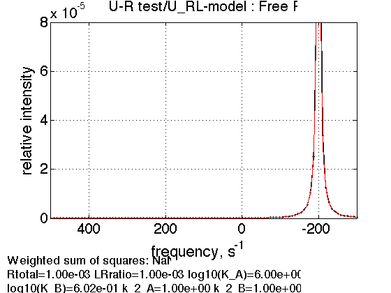
Single peak as expected.
Prepare TotalFit session for easy display of many graphs
storage_session=TotalFit('All_tests');
% set aside for plotting later
storage_session.copy_dataset_into_array(test1);
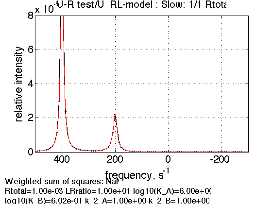
2. Saturated receptor
% Use the same thermodynamic parameters as above. Add spectral and kinetic parameters:
LRratio = 10 ;

% compute equilbrium concentrations
[concentrations species_names] = equilibrium_thermodynamic_equations.U_RL_model(...
        Rtotal, LRratio, K_a_A, K_a_B,...
        model_numeric_solver, model_numeric_options)


% plot line shapes
parameters=[ Rtotal  LRratio   Log10_K_A   Log10_K_B  k_2_A  k_2_B ...
     w0_R  w0_RL  w0_RLstar  FWHH_R  FWHH_RL  FWHH_RLstar  ScaleFactor ];


test1.simulate_noisy_data(parameters, X_RMSD, Y_RMSD);
figure_handle=test1.plot_simulation('Slow: 1/1 Rtotal');
results_output.output_figure(figure_handle, figures_folder, 'Slow_concentrated_R');
% set aside
storage_session.copy_dataset_into_array(test1);
concentrations =

    0.0000    0.0002    0.0008    0.0090


species_names =

    'Req'    'RLeq'    'RLstareq'    'Leq'
3. Dilution of the complex
Rtotal=1e-4;

% compute equilbrium concentrations
[concentrations species_names] = equilibrium_thermodynamic_equations.U_RL_model(...
        Rtotal, LRratio, K_a_A, K_a_B,...
        model_numeric_solver, model_numeric_options)


parameters=[ Rtotal  LRratio   Log10_K_A   Log10_K_B  k_2_A  k_2_B ...
     w0_R  w0_RL  w0_RLstar  FWHH_R  FWHH_RL  FWHH_RLstar  ScaleFactor ];


test1.simulate_noisy_data(parameters, X_RMSD, Y_RMSD);
figure_handle=test1.plot_simulation('Slow: 1/10 R');
results_output.output_figure(figure_handle, figures_folder, 'Slow_diluted_R');

% set aside
storage_session.copy_dataset_into_array(test1);
concentrations =

   1.0e-03 *

    0.0000    0.0200    0.0800    0.9000


species_names =

    'Req'    'RLeq'    'RLstareq'    'Leq'
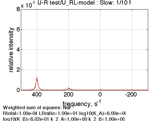
As expected, there is no change in ratio between peak areas.
4. Fast exchange in the complex
Rtotal=1e-3;
k_2_B=1000;

% compute equilbrium concentrations
[concentrations species_names] = equilibrium_thermodynamic_equations.U_RL_model(...
        Rtotal, LRratio, K_a_A, K_a_B,...
        model_numeric_solver, model_numeric_options)


parameters=[ Rtotal  LRratio   Log10_K_A   Log10_K_B  k_2_A  k_2_B ...
     w0_R  w0_RL  w0_RLstar  FWHH_R  FWHH_RL  FWHH_RLstar  ScaleFactor ];


test1.simulate_noisy_data(parameters, X_RMSD, Y_RMSD);
figure_handle=test1.plot_simulation('Fast isom.');
results_output.output_figure(figure_handle, figures_folder, 'Fast_isomerization');

% set aside
storage_session.copy_dataset_into_array(test1);
concentrations =

    0.0000    0.0002    0.0008    0.0090


species_names =

    'Req'    'RLeq'    'RLstareq'    'Leq'
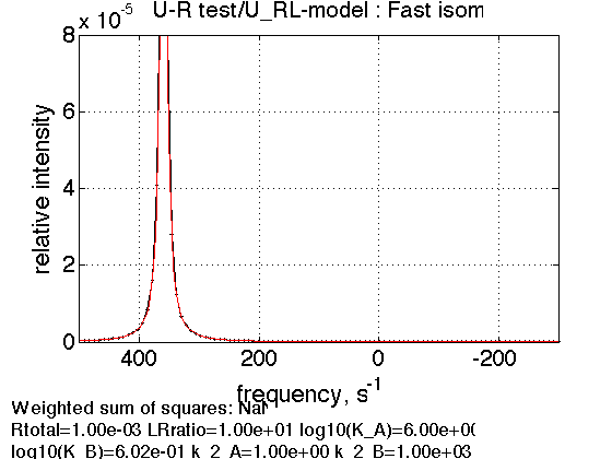
Peak appears at 1/5 of the distance between RL and RL* frequencies in favor of RL* as expected.
5. Fast exchange in the diluted complex
Rtotal=1e-4;


% compute equilbrium concentrations
[concentrations species_names] = equilibrium_thermodynamic_equations.U_RL_model(...
        Rtotal, LRratio, K_a_A, K_a_B,...
        model_numeric_solver, model_numeric_options)


parameters=[ Rtotal  LRratio   Log10_K_A   Log10_K_B  k_2_A  k_2_B ...
     w0_R  w0_RL  w0_RLstar  FWHH_R  FWHH_RL  FWHH_RLstar  ScaleFactor ];


test1.simulate_noisy_data(parameters, X_RMSD, Y_RMSD);
figure_handle=test1.plot_simulation('Fast isom.');
results_output.output_figure(figure_handle, figures_folder, 'Fast_isomerization');

% set aside
storage_session.copy_dataset_into_array(test1);
concentrations =

   1.0e-03 *

    0.0000    0.0200    0.0800    0.9000


species_names =

    'Req'    'RLeq'    'RLstareq'    'Leq'
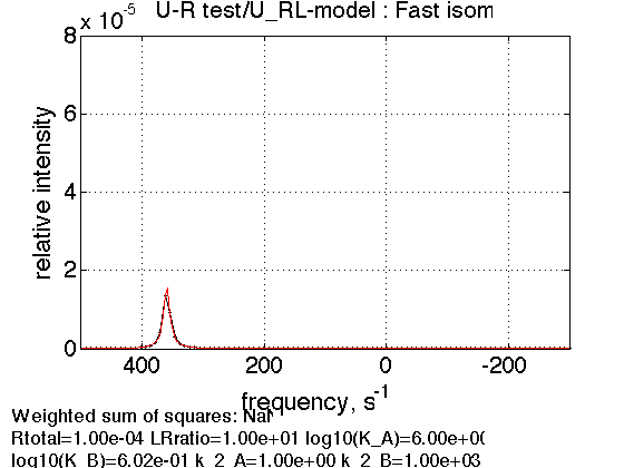
Peak still appears at 1/5 of the distance between RL and RL* frequencies in favor of RL* confirming the isomerization equlibrium is not dependent on receptor complex concentration
Summary of individual plots
storage_session.define_series('All-tests',1:length(storage_session.dataset_array));
figure_handle=storage_session.plot_1D_series('All-tests', 'All tests', 0);
results_output.output_figure(figure_handle, figures_folder, 'All_tests');
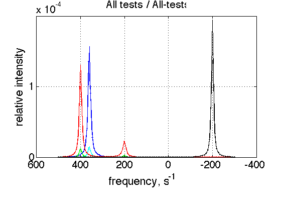
This is a comparison graph of all previous plots
Create a titration series
(see Tutorial 3 for details) Choose parameters
ZERO_LRratio= 1e-3; % This number should not be zero
LRratio_vector=[ZERO_LRratio  0.2   0.4   0.6  0.8   1.0   1.2   1.4 ];
k_2_A=1000;
k_2_B=10;


% choose the same parameters as above
session_name='Series';
session=TotalFit(session_name);
series_name='U-RL_simulation';
dataset_class_name='NMRLineShapes1D';
model_name='U_RL-model';
number_of_datasets=length(LRratio_vector);
X_column=test1.X; % use the same range

% create TotalFit session
session.create_simulation_series(series_name, dataset_class_name, model_name, ...
                 model_numeric_solver, model_numeric_options,...
                 number_of_datasets, X_column);

session.initialize_relation_matrix(sprintf('%s.all_datasets.txt', session_name));

% link parameters
parameter_number_array=[ 1    3 4 5 6 7 8 9 10 11 12 13];
session.batch_link_parameters_in_series(series_name, parameter_number_array);
session.generate_fitting_environment(sprintf('%s.fitting_environment.txt', session_name))

% prepare parameters
first_dataset_index=session.dataset_index(series_name,1);
FAKE_VALUE=1E-6;  % individual (unlinked) parameters: to be assigned later

ideal_parameters=[ Rtotal  FAKE_VALUE   Log10_K_A   Log10_K_B  k_2_A  k_2_B ...
     w0_R  w0_RL  w0_RLstar  FWHH_R  FWHH_RL  FWHH_RLstar  ScaleFactor ];

% prepare formal limits
fake_limits=zeros(1,length(ideal_parameters));
Monte_Carlo_range_min=fake_limits;
Monte_Carlo_range_max=fake_limits;
parameter_limits_min=fake_limits;
parameter_limits_max=fake_limits;

% assign
session.assign_parameter_values(first_dataset_index, ideal_parameters, ...
        Monte_Carlo_range_min, Monte_Carlo_range_max, parameter_limits_min, parameter_limits_max);

% Assign unlinked LRratio and ranges
parameter_number=2;
values_array=LRratio_vector;

unlinked_fake_ranges=zeros(1,number_of_datasets);
MonteCarlo_range_min_array=unlinked_fake_ranges;
MonteCarlo_range_max_array=unlinked_fake_ranges;
parameter_limits_min_array=unlinked_fake_ranges;
parameter_limits_max_array=unlinked_fake_ranges;

session.assign_unlinked_parameter_in_series(...
             series_name, parameter_number, values_array, ...
             MonteCarlo_range_min_array, MonteCarlo_range_max_array, ...
             parameter_limits_min_array, parameter_limits_max_array);

% Simulate series
X_standard_dev=0;
Y_standard_dev=1e-8;  % something really small
session.simulate_series(series_name, X_standard_dev, Y_standard_dev);

% Plot
Y_offset_percent=10;  % to offset figures vertically for easier viewing
% set plotting ranges
X_range=test1.X_range;  % use old
Y_range=[];  % automatic
session.set_XY_ranges_series(series_name, X_range, Y_range)
figure_handle=session.plot_1D_series(series_name, session.name, Y_offset_percent);
results_output.output_figure(figure_handle, figures_folder, 'Series');
Dataset listing is written to "Series.all_datasets.txt".

Fitting environment saved in Series.fitting_environment.txt.

ans =

New parameter relations (indexed as in all_parameters vector):

[1]     1:Rtotal | 2:Rtotal | 3:Rtotal | 4:Rtotal | 5:Rtotal | 6:Rtotal | 7:Rtotal | 8:Rtotal
[2]     1:LRratio
[3]     1:log10(K_A) | 2:log10(K_A) | 3:log10(K_A) | 4:log10(K_A) | 5:log10(K_A) | 6:log10(K_A) | 7:log10(K_A) | 8:log10(K_A)
[4]     1:log10(K_B) | 2:log10(K_B) | 3:log10(K_B) | 4:log10(K_B) | 5:log10(K_B) | 6:log10(K_B) | 7:log10(K_B) | 8:log10(K_B)
[5]     1:k_2_A | 2:k_2_A | 3:k_2_A | 4:k_2_A | 5:k_2_A | 6:k_2_A | 7:k_2_A | 8:k_2_A
[6]     1:k_2_B | 2:k_2_B | 3:k_2_B | 4:k_2_B | 5:k_2_B | 6:k_2_B | 7:k_2_B | 8:k_2_B
[7]     1:w0_R | 2:w0_R | 3:w0_R | 4:w0_R | 5:w0_R | 6:w0_R | 7:w0_R | 8:w0_R
[8]     1:w0_RL | 2:w0_RL | 3:w0_RL | 4:w0_RL | 5:w0_RL | 6:w0_RL | 7:w0_RL | 8:w0_RL
[9]     1:w0_RLstar | 2:w0_RLstar | 3:w0_RLstar | 4:w0_RLstar | 5:w0_RLstar | 6:w0_RLstar | 7:w0_RLstar | 8:w0_RLstar
[10]     1:FWHH_R | 2:FWHH_R | 3:FWHH_R | 4:FWHH_R | 5:FWHH_R | 6:FWHH_R | 7:FWHH_R | 8:FWHH_R
[11]     1:FWHH_RL | 2:FWHH_RL | 3:FWHH_RL | 4:FWHH_RL | 5:FWHH_RL | 6:FWHH_RL | 7:FWHH_RL | 8:FWHH_RL
[12]     1:FWHH_RLstar | 2:FWHH_RLstar | 3:FWHH_RLstar | 4:FWHH_RLstar | 5:FWHH_RLstar | 6:FWHH_RLstar | 7:FWHH_RLstar | 8:FWHH_RLstar
[13]     1:ScaleFactor | 2:ScaleFactor | 3:ScaleFactor | 4:ScaleFactor | 5:ScaleFactor | 6:ScaleFactor | 7:ScaleFactor | 8:ScaleFactor
[14]   n/a
[15]     2:LRratio
[16]   n/a
[17]   n/a
[18]   n/a
[19]   n/a
[20]   n/a
[21]   n/a
[22]   n/a
[23]   n/a
[24]   n/a
[25]   n/a
[26]   n/a
[27]   n/a
[28]     3:LRratio
[29]   n/a
[30]   n/a
[31]   n/a
[32]   n/a
[33]   n/a
[34]   n/a
[35]   n/a
[36]   n/a
[37]   n/a
[38]   n/a
[39]   n/a
[40]   n/a
[41]     4:LRratio
[42]   n/a
[43]   n/a
[44]   n/a
[45]   n/a
[46]   n/a
[47]   n/a
[48]   n/a
[49]   n/a
[50]   n/a
[51]   n/a
[52]   n/a
[53]   n/a
[54]     5:LRratio
[55]   n/a
[56]   n/a
[57]   n/a
[58]   n/a
[59]   n/a
[60]   n/a
[61]   n/a
[62]   n/a
[63]   n/a
[64]   n/a
[65]   n/a
[66]   n/a
[67]     6:LRratio
[68]   n/a
[69]   n/a
[70]   n/a
[71]   n/a
[72]   n/a
[73]   n/a
[74]   n/a
[75]   n/a
[76]   n/a
[77]   n/a
[78]   n/a
[79]   n/a
[80]     7:LRratio
[81]   n/a
[82]   n/a
[83]   n/a
[84]   n/a
[85]   n/a
[86]   n/a
[87]   n/a
[88]   n/a
[89]   n/a
[90]   n/a
[91]   n/a
[92]   n/a
[93]     8:LRratio
[94]   n/a
[95]   n/a
[96]   n/a
[97]   n/a
[98]   n/a
[99]   n/a
[100]   n/a
[101]   n/a
[102]   n/a
[103]   n/a
[104]   n/a

Summary of datasets with lookup vectors (position of each parameter in all_parameter vector)
--------
Dataset 1/U-RL_simulation-1,  model "U_RL-model"
Parameters          :    Rtotal    LRratio    log10(K_A)    log10(K_B)    k_2_A    k_2_B    w0_R    w0_RL    w0_RLstar    FWHH_R    FWHH_RL    FWHH_RLstar    ScaleFactor
Lookup vector       :   1   2   3   4   5   6   7   8   9   10   11   12   13

Dataset 2/U-RL_simulation-2,  model "U_RL-model"
Parameters          :    Rtotal    LRratio    log10(K_A)    log10(K_B)    k_2_A    k_2_B    w0_R    w0_RL    w0_RLstar    FWHH_R    FWHH_RL    FWHH_RLstar    ScaleFactor
Lookup vector       :   1   15   3   4   5   6   7   8   9   10   11   12   13

Dataset 3/U-RL_simulation-3,  model "U_RL-model"
Parameters          :    Rtotal    LRratio    log10(K_A)    log10(K_B)    k_2_A    k_2_B    w0_R    w0_RL    w0_RLstar    FWHH_R    FWHH_RL    FWHH_RLstar    ScaleFactor
Lookup vector       :   1   28   3   4   5   6   7   8   9   10   11   12   13

Dataset 4/U-RL_simulation-4,  model "U_RL-model"
Parameters          :    Rtotal    LRratio    log10(K_A)    log10(K_B)    k_2_A    k_2_B    w0_R    w0_RL    w0_RLstar    FWHH_R    FWHH_RL    FWHH_RLstar    ScaleFactor
Lookup vector       :   1   41   3   4   5   6   7   8   9   10   11   12   13

Dataset 5/U-RL_simulation-5,  model "U_RL-model"
Parameters          :    Rtotal    LRratio    log10(K_A)    log10(K_B)    k_2_A    k_2_B    w0_R    w0_RL    w0_RLstar    FWHH_R    FWHH_RL    FWHH_RLstar    ScaleFactor
Lookup vector       :   1   54   3   4   5   6   7   8   9   10   11   12   13

Dataset 6/U-RL_simulation-6,  model "U_RL-model"
Parameters          :    Rtotal    LRratio    log10(K_A)    log10(K_B)    k_2_A    k_2_B    w0_R    w0_RL    w0_RLstar    FWHH_R    FWHH_RL    FWHH_RLstar    ScaleFactor
Lookup vector       :   1   67   3   4   5   6   7   8   9   10   11   12   13

Dataset 7/U-RL_simulation-7,  model "U_RL-model"
Parameters          :    Rtotal    LRratio    log10(K_A)    log10(K_B)    k_2_A    k_2_B    w0_R    w0_RL    w0_RLstar    FWHH_R    FWHH_RL    FWHH_RLstar    ScaleFactor
Lookup vector       :   1   80   3   4   5   6   7   8   9   10   11   12   13

Dataset 8/U-RL_simulation-8,  model "U_RL-model"
Parameters          :    Rtotal    LRratio    log10(K_A)    log10(K_B)    k_2_A    k_2_B    w0_R    w0_RL    w0_RLstar    FWHH_R    FWHH_RL    FWHH_RLstar    ScaleFactor
Lookup vector       :   1   93   3   4   5   6   7   8   9   10   11   12   13
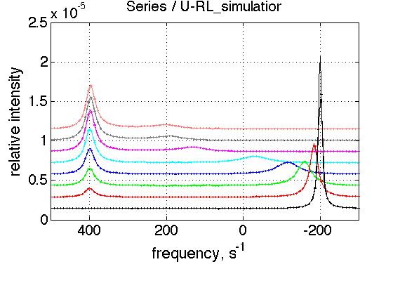
This is expected result. Weighted average peak between R and RL moves towards RL and diminishes as contribution from R reduces.
CONCLUSIONS
The U-RL model of 1D NMR line shape works.