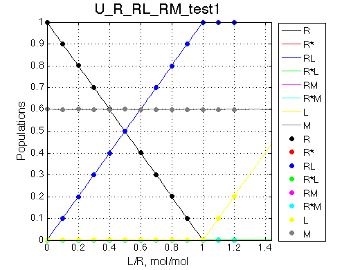
Equilibrium molar fractions of species Points correspond to steps in titration series corresponding to Rtotal and LRratio used in NMR line shape simulations below. Curves are smooth functions simulated at constant Rtotal. Populations of multimeric species are shown per monomer. Population of free ligand is normalized to total receptor concentration. |
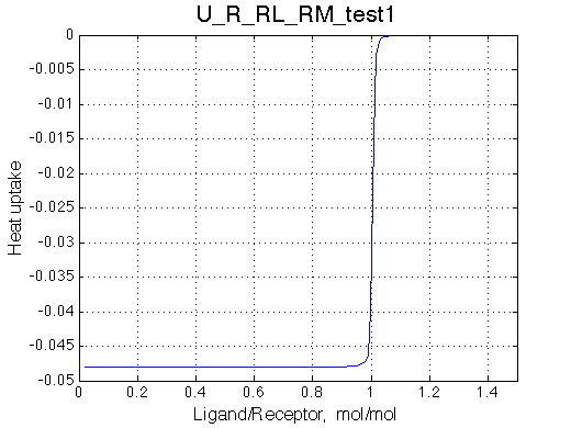
Isothermal Titration Calorimetry profile Heat uptake curve is simulated as a derivative of the population of species multiplied by specific dH. |
U_R_RL_RM_test1 |
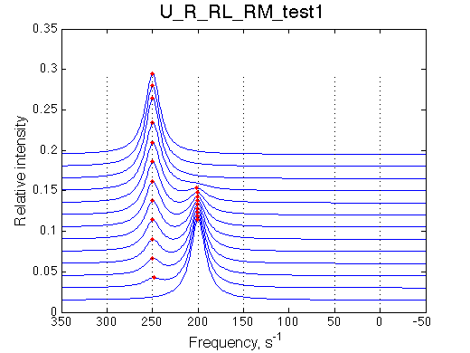
1D-spectra of the titration series Traces (bottom to top) correspond to L/R ratios indicated by points in the Populations graph (above). Red dots indicate peak maxima for a visual aid (also plotted as the chemical shift titration curves on the right). Dashed lines indicate chemical shifts of individual species. |
Chemical shift titration curves Points correspond to positions of peak maxima numerically detected in the spectral traces. Sometimes not all peaks will be detected and signal/noise here is not considered. |
|
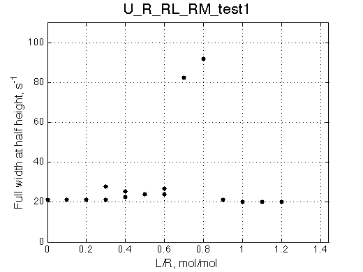
| Plot of the line widths (full width at a half height)
Plain text data for comparison plotting: TXT The full width at a half height (FWHH) is determined numerically for the detected peaks. For the lorentzian line shape FWHH = 2*R2. |
Equilibrium molar fractions of species Points correspond to steps in titration series corresponding to Rtotal and LRratio used in NMR line shape simulations below. Curves are smooth functions simulated at constant Rtotal. Populations of multimeric species are shown per monomer. Population of free ligand is normalized to total receptor concentration. |
Isothermal Titration Calorimetry profile Heat uptake curve is simulated as a derivative of the population of species multiplied by specific dH. |
U_R_RL_RM_test2 |
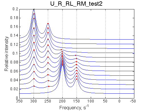
1D-spectra of the titration series Traces (bottom to top) correspond to L/R ratios indicated by points in the Populations graph (above). Red dots indicate peak maxima for a visual aid (also plotted as the chemical shift titration curves on the right). Dashed lines indicate chemical shifts of individual species. |
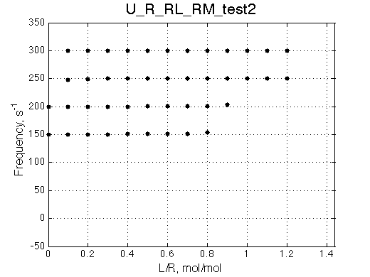
Chemical shift titration curves Points correspond to positions of peak maxima numerically detected in the spectral traces. Sometimes not all peaks will be detected and signal/noise here is not considered. |
|
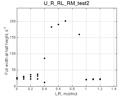
| Plot of the line widths (full width at a half height)
Plain text data for comparison plotting: TXT The full width at a half height (FWHH) is determined numerically for the detected peaks. For the lorentzian line shape FWHH = 2*R2. |
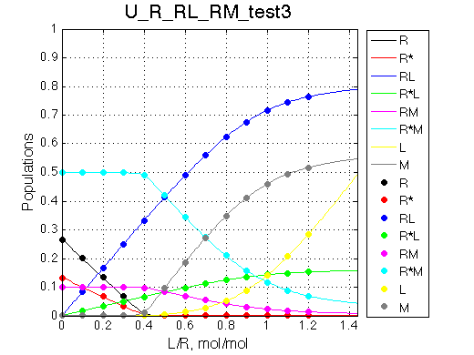
Equilibrium molar fractions of species Points correspond to steps in titration series corresponding to Rtotal and LRratio used in NMR line shape simulations below. Curves are smooth functions simulated at constant Rtotal. Populations of multimeric species are shown per monomer. Population of free ligand is normalized to total receptor concentration. |
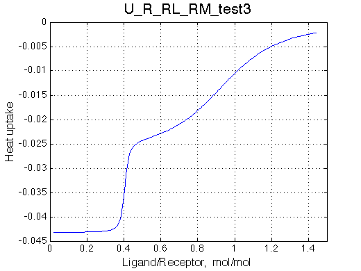
Isothermal Titration Calorimetry profile Heat uptake curve is simulated as a derivative of the population of species multiplied by specific dH. |
U_R_RL_RM_test3 |
1D-spectra of the titration series Traces (bottom to top) correspond to L/R ratios indicated by points in the Populations graph (above). Red dots indicate peak maxima for a visual aid (also plotted as the chemical shift titration curves on the right). Dashed lines indicate chemical shifts of individual species. |
Chemical shift titration curves Points correspond to positions of peak maxima numerically detected in the spectral traces. Sometimes not all peaks will be detected and signal/noise here is not considered. |
|
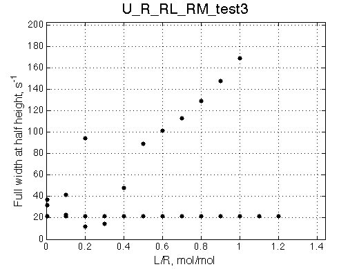
| Plot of the line widths (full width at a half height)
Plain text data for comparison plotting: TXT The full width at a half height (FWHH) is determined numerically for the detected peaks. For the lorentzian line shape FWHH = 2*R2. |
Equilibrium molar fractions of species Points correspond to steps in titration series corresponding to Rtotal and LRratio used in NMR line shape simulations below. Curves are smooth functions simulated at constant Rtotal. Populations of multimeric species are shown per monomer. Population of free ligand is normalized to total receptor concentration. |
Isothermal Titration Calorimetry profile Heat uptake curve is simulated as a derivative of the population of species multiplied by specific dH. |
U_R_RL_RM_test4 |
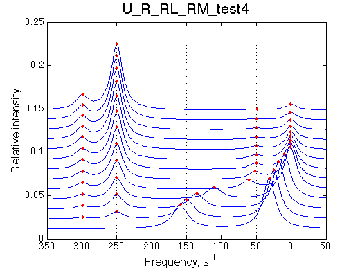
1D-spectra of the titration series Traces (bottom to top) correspond to L/R ratios indicated by points in the Populations graph (above). Red dots indicate peak maxima for a visual aid (also plotted as the chemical shift titration curves on the right). Dashed lines indicate chemical shifts of individual species. |
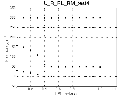
Chemical shift titration curves Points correspond to positions of peak maxima numerically detected in the spectral traces. Sometimes not all peaks will be detected and signal/noise here is not considered. |
|
| Plot of the line widths (full width at a half height)
Plain text data for comparison plotting: TXT The full width at a half height (FWHH) is determined numerically for the detected peaks. For the lorentzian line shape FWHH = 2*R2. |
LineShapeKin Simulation
Evgenii Kovrigin, Medical College of Wisconsin, 2009