NMR line shape simulation mode

You may simulate line shapes for a specific peak for different possible combinations of parameters. You need titration spectral data for that as a simulation uses real frequency ranges from these data. You may do simulation using fully manually entered starting parameters or let the program determine peak positions and relaxation rates and then you may vary the kinetic and equilibrium constants to see the effect.
In order to do this :
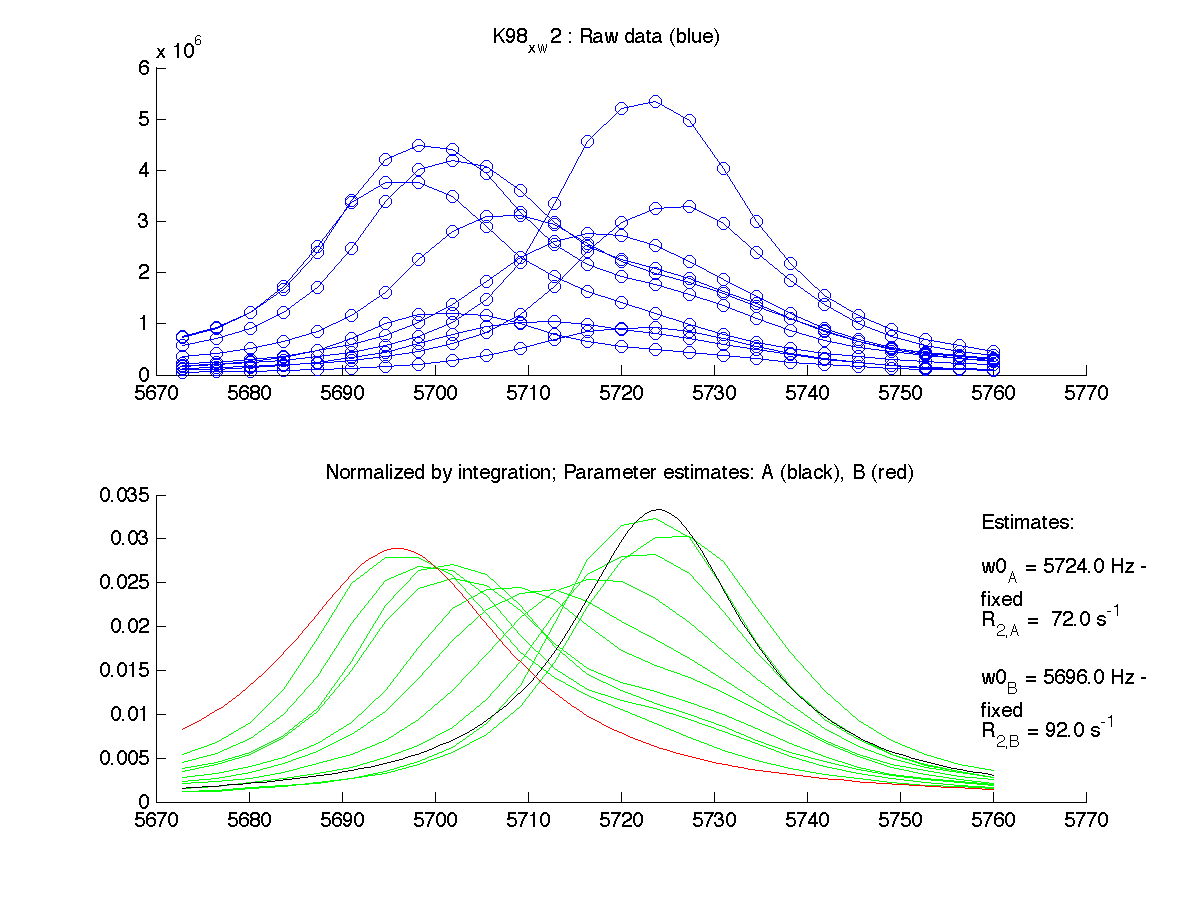
- Slice the peak region in Sparky
- enter dataset name in resnames (setup.m)
- Now you have a choice to either
  - set up frequencies and relaxation rates entirely manually, or
  - let the program estimate them for your current peak and use them in simulation (you will only provide K_d and k_off values then)
- (1) Fully manual simulation:
  - Enter desired
    - frequencies (Hz) in manual_w0.txt as a column
      start_w0
      end_w0
    - relaxation rate (/s) in manual_R2.txt (remember, they will be much larger in you spectral data sets then real ones because of finite acquisition time and application of EM window )
  - set project_name='simulation' (setup.m)
  - Enter desired K_d, k_off etc in model_setup.m
    - Model.Kd
    - Model.Koff
    - etc
  - issue main
- (2) Simulation using peak positions and line widths of real signals
  - set project_name='just display data' (setup.m)
  - issue main and make sure the estimates for starting and ending points look good
  - set project_name='simulation' (setup.m)
  - Enter desired K_d, k_off etc in model_setup.m
    - Model.Kd
    - Model.Koff
    - ...
  - issue main
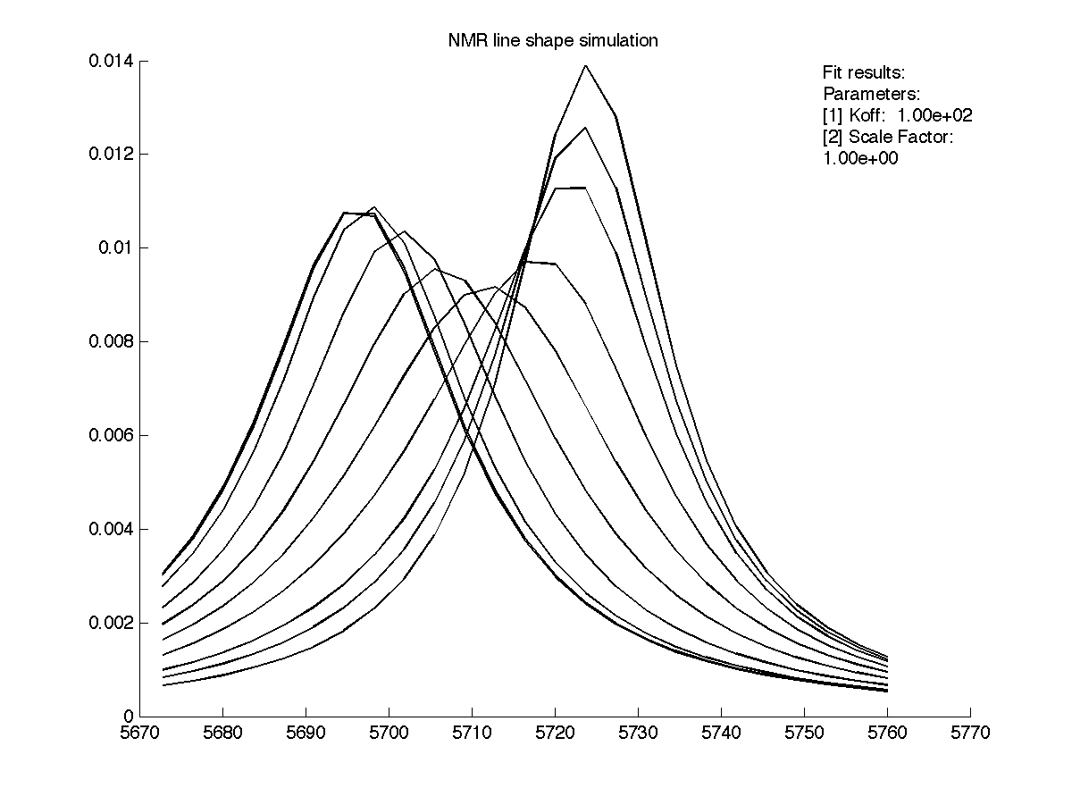
- The program shows two graphs - raw data and simulation results. It saves them in figures/ as both PNG image and FIG file editable in Matlab.
  
  K98_x_w2_normalization.png simulation.png

Back to the Contents

K98_x_w2_normalization.png	simulation.png