

Here we will compare outcomes of the four alternative models for conditions when binding is very slow while isomerization is in intermediate exchange. I choose binding affinity of 108 M-1 and off-rate of 1 s-1. R and RL are separated by 100 s-1 and R* or R*L - by 100 s-1 from corresponding species. Isomerization equilibrium is shifted 5:1 toward *-forms and occurs in intermediate exchange with kex equal to the the chemical shift separation of the alternative conformations: 100 s-1 and the corresponding reverse rate: 100*1/6=17 s-1.
Location: As_Bi/
|
|
|
|
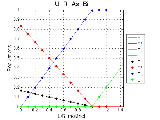
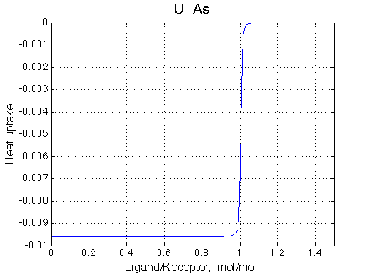
| U_As.txt | U_R_As_Bi.txt | U_L_As_Bi.txt | U_RL_As_Bi.txt |
|
|
|
|
|
|
|
|
|
|
|
|
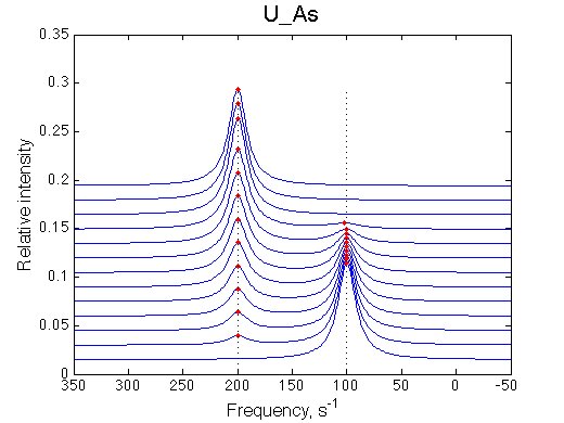
Exchange between alternative conformations is intermediate, so we don't see the peak of minor conformation any more. The system looks quite unpromising in terms of our ability to detect coupled conformational exchange. However, we may use fitting of this data with the U model as a research tool and observe effects on apparent Kd and koff .
Hypothesis: The key phenomenon we may exploit in analysis of this slow/intermediate-exchange system is the dependence of the fitted apparent Kd on the chemical shift separation between the peaks.
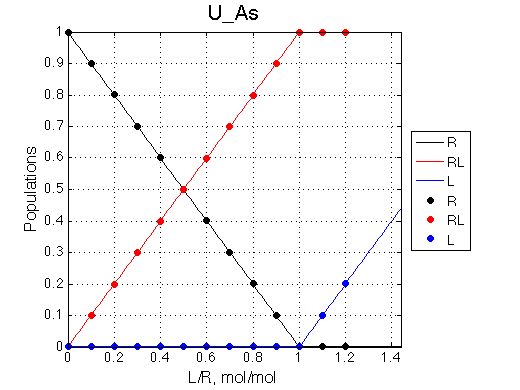
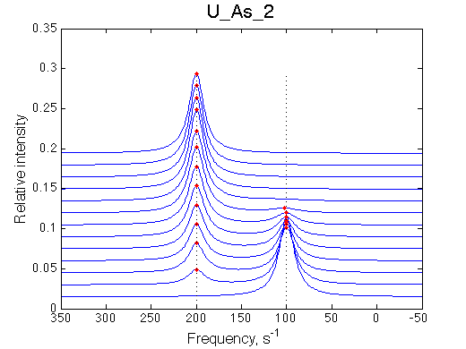
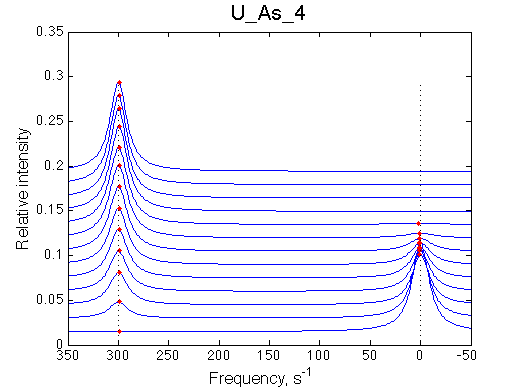
First we need to test the performance of the LineShapeKin 3 fitting algorithm using simulated data with the variable peak separation. We need to see how much the fitting quality is dependent on the separation between resonances.
50 s-1 |
100 s-1 |
200 s-1 |
300 s-1 |
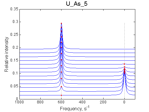
600 s-1 | 900 s-1 | |
| U_As_1 | U_As_2 | U_As_3 | U_As_4 | Simulate setup_wide U_As_5 | Simulate setup_wide U_As_6 | |
 |
 |
 |
 |
 |
 |
|
 |
 |
 |
 |
 |
 |
|
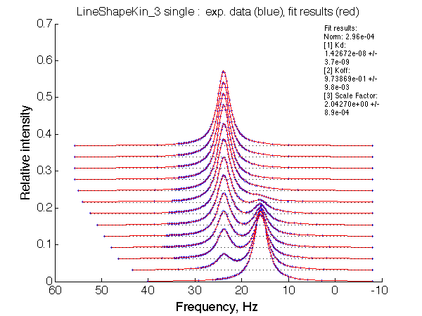
| Optimum norm: 2.96e-04 [1] Kd: 1.42672e-08 +/- 3.7e-09 [2] Koff: 9.73869e-01 +/- 9.8e-03 [3] Scale Factor: 2.04270e+00 +/- 8.9e-04 |
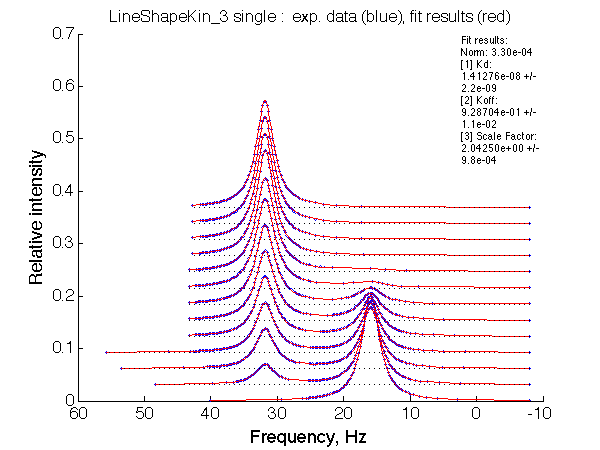
Optimum norm: 3.30e-04 [1] Kd: 1.41276e-08 +/- 2.2e-09 [2] Koff: 9.28704e-01 +/- 1.1e-02 [3] Scale Factor: 2.04250e+00 +/- 9.8e-04 |
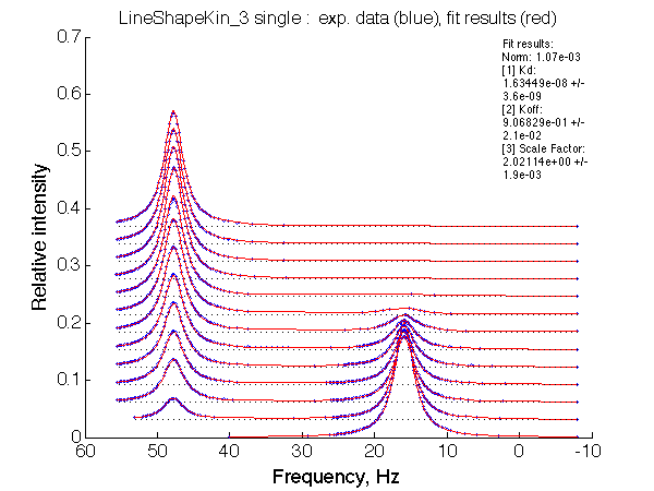
Optimum norm: 1.07e-03 [1] Kd: 1.63449e-08 +/- 3.6e-09 [2] Koff: 9.06829e-01 +/- 2.1e-02 [3] Scale Factor: 2.02114e+00 +/- 1.9e-03 |
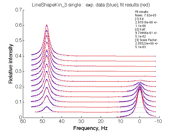
Optimum norm: 7.02e-03 [1] Kd: 2.97818e-08 +/- 1.1e-08 [2] Koff: 9.73446e-01 +/- 5.1e-02 [3] Scale Factor: 2.05523e+00 +/- 5.1e-03 |
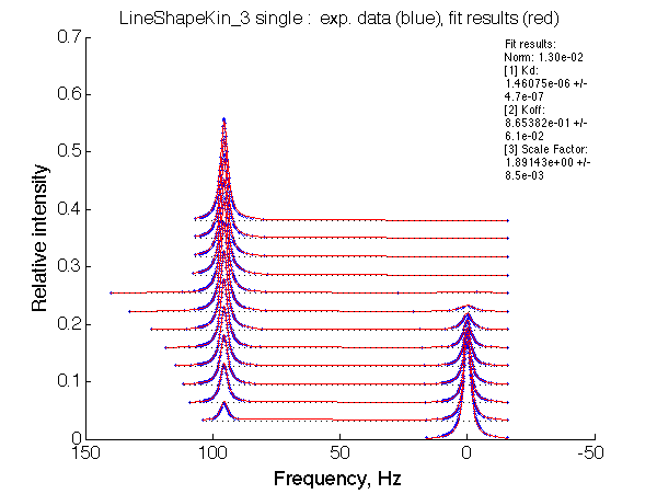
Optimum norm: 1.30e-02 [1] Kd: 1.46075e-06 +/- 4.7e-07 [2] Koff: 8.65382e-01 +/- 6.1e-02 [3] Scale Factor: 1.89143e+00 +/- 8.5e-03 |
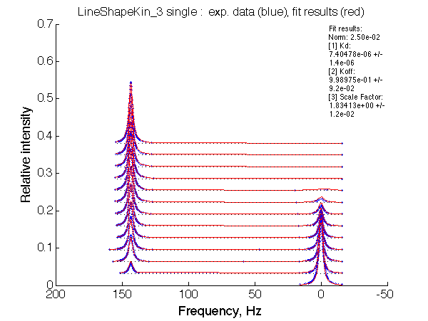
LSQCURVFIT converged to a solution Determination of parameter uncertainties... Norm (sum of squared residuals): 2.50e-02 [1] Kd: 7.40478e-06 +/- 1.4e-06 [2] Koff: 9.98975e-01 +/- 9.2e-02 [3] Scale Factor: 1.83413e+00 +/- 1.2e-02 |
I collect these numbers in summary_Kdvsw.txt and plot with
plotdatasets 'Fit_quality' 'Chemical shift separation, s^{-1}' 'K_d, M'

A note on fitting quality: Fitting result is quite stable to about 300 s-1. Pre-set Kd was 1*10-8. After that the fit quality degrades and that is manifested by deviation of the fitted Kd from the preset Kd value.
Common parameters we use are:
# Association constants
Ka_names A B
Ka 1e8 5
# Rate constants of REVERSE reactions
k_names A B
k2 1 25
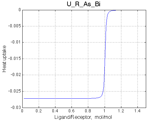
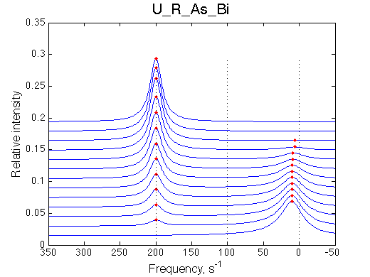
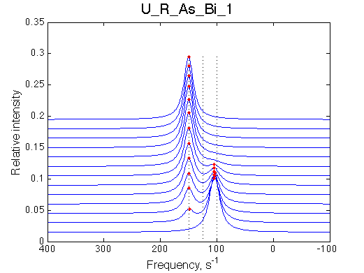
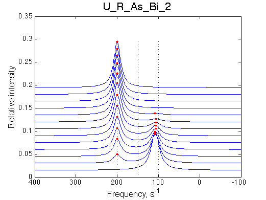
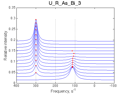
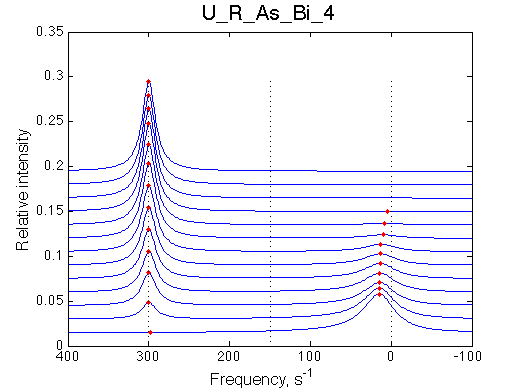
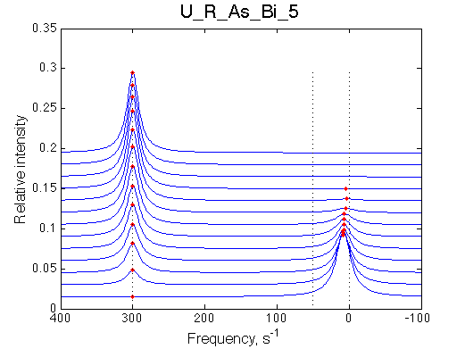
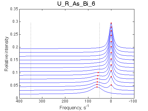
| between peaks/dw(B) | 50/25 | 100/50 | 200/100 | 300/150 | 300/50 | 50/300 |
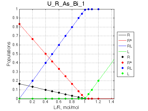
Simulate setup U_R_As_Bi_1 |
Simulate setup U_R_As_Bi_2 |
Simulate setup U_R_As_Bi_3 |
Simulate setup U_R_As_Bi_4 |
Simulate setup U_R_As_Bi_5 |
Simulate setup U_R_As_Bi_6 | |
 |
 |
 |
 |
 |
 |
|
 |
 |
 |
 |
 |
 |
|
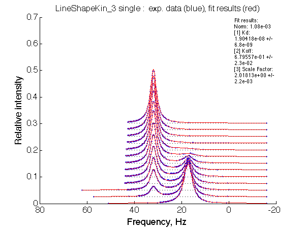
| LSQCURVFIT converged to a solution Determination of parameter uncertainties... Norm (sum of squared residuals): 6.07e-04 [1] Kd: 2.83848e-08 +/- 9.4e-09 [2] Koff: 7.56248e-01 +/- 1.7e-02 [3] Scale Factor: 2.00888e+00 +/- 1.5e-03 |
Maximum number of iterations reached! Determination of parameter uncertainties... Norm (sum of squared residuals): 1.18e-03 [1] Kd: 1.58792e-08 +/- 5.3e-09 [2] Koff: 6.97622e-01 +/- 2.0e-02 [3] Scale Factor: 2.04771e+00 +/- 1.9e-03 |
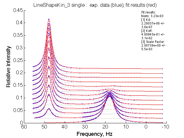
LSQCURVFIT converged to a solution Determination of parameter uncertainties... Norm (sum of squared residuals): 3.23e-03 [1] Kd: 2.28037e-06 +/- 3.6e-07 [2] Koff: 4.80843e-01 +/- 3.1e-02 [3] Scale Factor: 2.08739e+00 +/- 5.5e-03 |
LSQCURVFIT converged to a solution Determination of parameter uncertainties... Norm (sum of squared residuals): 5.65e-03 [1] Kd: 1.51640e-05 +/- 1.2e-06 [2] Koff: 5.22583e-01 +/- 4.4e-02 [3] Scale Factor: 2.20645e+00 +/- 8.8e-03 |
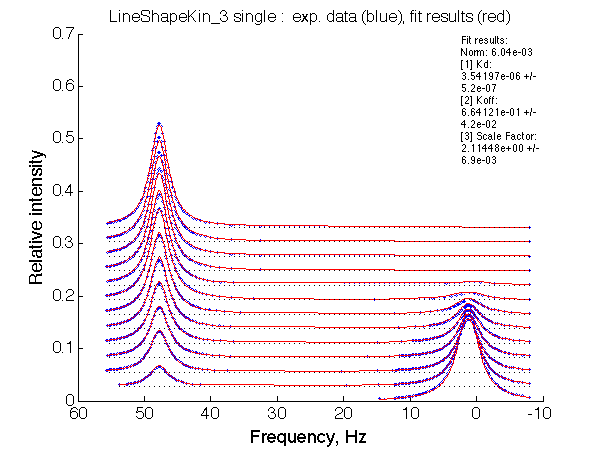
LSQCURVFIT converged to a solution Determination of parameter uncertainties... Norm (sum of squared residuals): 6.04e-03 [1] Kd: 3.54197e-06 +/- 5.2e-07 [2] Koff: 6.64121e-01 +/- 4.2e-02 [3] Scale Factor: 2.11448e+00 +/- 6.9e-03 |
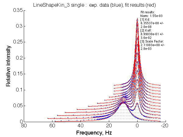
LSQCURVFIT converged to a solution Determination of parameter uncertainties... Norm (sum of squared residuals): 1.55e-03 [1] Kd: 6.35537e-08 +/- 2.0e-08 [2] Koff: 8.99030e-01 +/- 3.6e-02 [3] Scale Factor: 2.11083e+00 +/- 2.8e-03 |
Summarize Kd vs. dw in summary_Kdvsw.txt
plotdatasets 'Fit_quality' 'Chemical shift separation, s^{-1}' 'K_d, M'
move files to U_R/
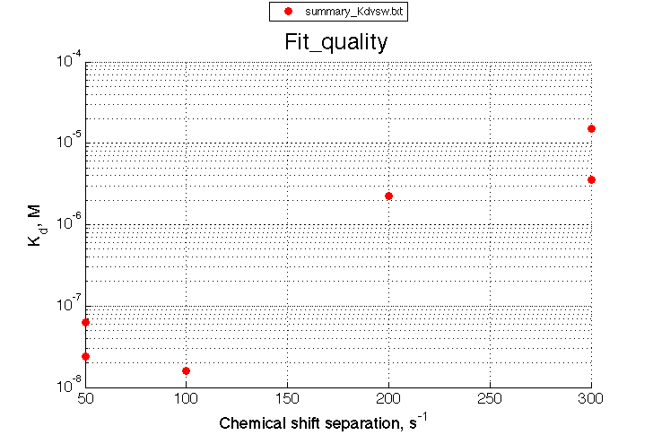
We observe a very remarkable phenomenon. The line shapes at the larger chemical shift separations resemble 2-site exchange less so the fit quality becomes progressively poorer. The apparent dissociation constant increases with dw very rapidly by 2-3-orders of magnitude at 300 s-1.
Important that it is chemical shift separation between R and RL what matters, not between R and R*.
Test the same common parameters:
# Association constants
Ka_names A B
Ka 1e8 5
# Rate constants of REVERSE reactions
k_names A B
k2 1 25
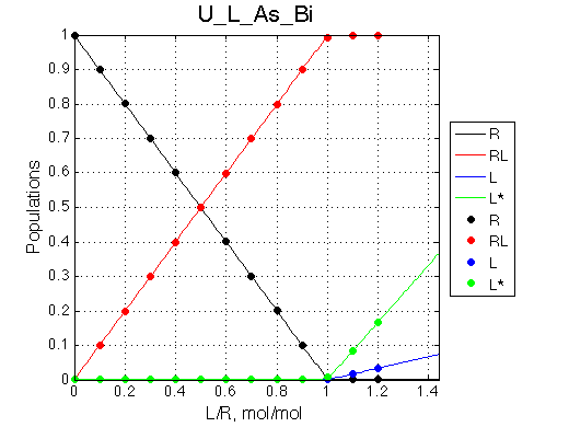
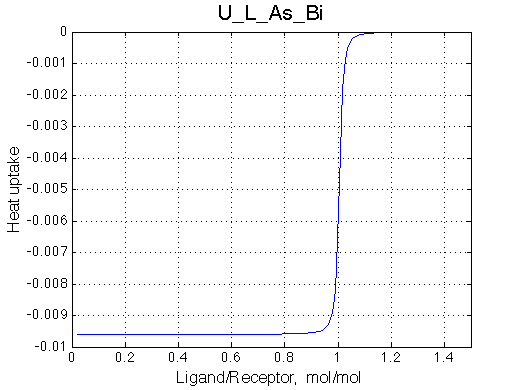
| between peaks/dw(B) | 50 | 100 | 200 | 300 |
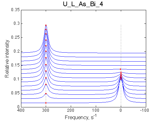
Simulate setup U_L_As_Bi_1 |
Simulate setup | Simulate setup U_L_As_Bi_3 | Simulate setup U_L_As_Bi_4 | |
 |
 |
 |
 |
|
 |
 |
 |
 |
|
| LSQCURVFIT converged to a solution Determination of parameter uncertainties... Norm (sum of squared residuals): 2.39e-04 [1] Kd: 6.61183e-08 +/- 7.7e-09 [2] Koff: 9.68117e-01 +/- 1.0e-02 [3] Scale Factor: 2.04040e+00 +/- 9.6e-04 |
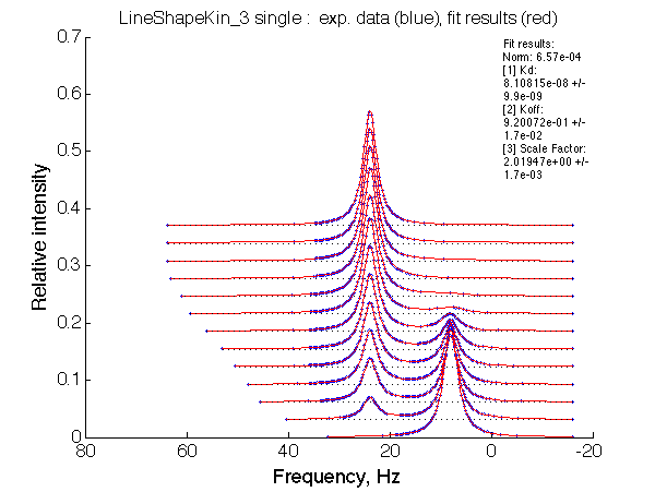
LSQCURVFIT converged to a solution Determination of parameter uncertainties... Norm (sum of squared residuals): 6.57e-04 [1] Kd: 8.10815e-08 +/- 9.9e-09 [2] Koff: 9.20072e-01 +/- 1.7e-02 [3] Scale Factor: 2.01947e+00 +/- 1.7e-03 |
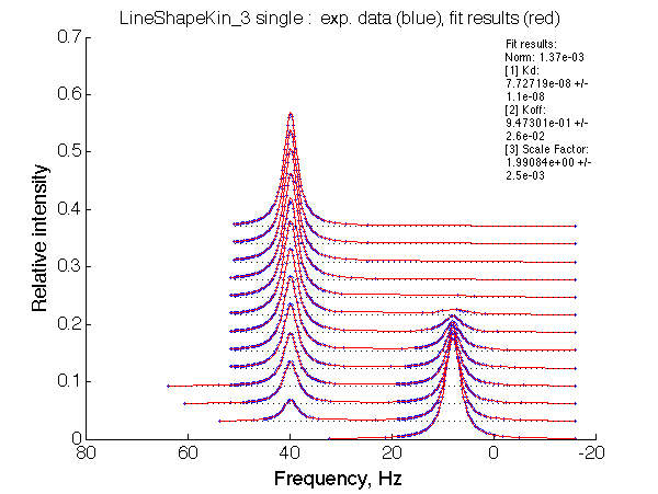
LSQCURVFIT converged to a solution Determination of parameter uncertainties... Norm (sum of squared residuals): 1.37e-03 [1] Kd: 7.72719e-08 +/- 1.1e-08 [2] Koff: 9.47301e-01 +/- 2.6e-02 [3] Scale Factor: 1.99084e+00 +/- 2.5e-03 |
LSQCURVFIT converged to a solution Determination of parameter uncertainties... Norm (sum of squared residuals): 3.08e-03 [1] Kd: 9.67200e-08 +/- 1.5e-08 [2] Koff: 9.77071e-01 +/- 3.9e-02 [3] Scale Factor: 1.98327e+00 +/- 3.9e-03 |
Summarize Kd vs. dw in summary_Kdvsw_U_L.txt
plotdatasets 'Fit_quality' 'Chemical shift separation, s^{-1}' 'K_d, M'
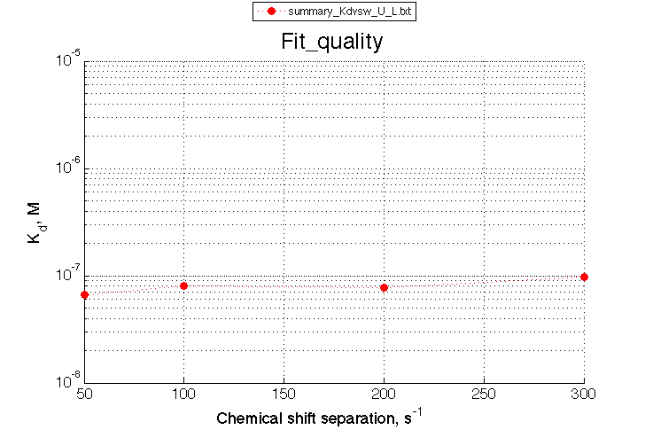
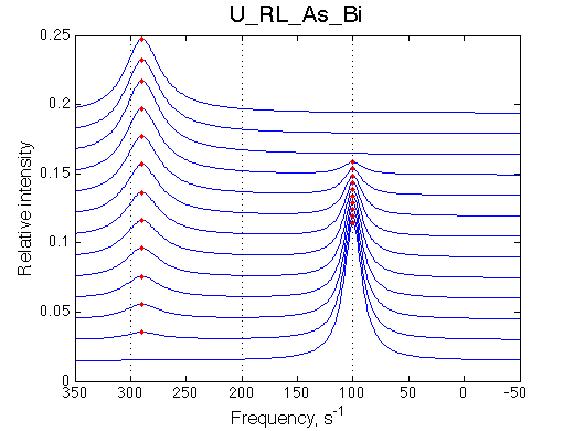
It is remarkable that the reverse titration of the U_R system produces very consistent Kd over a range of chemical shifts.
It may be predicted that if we can fit line shapes to obtain Kd for a number of sites in the ligand and the receptor, then due to intrinsic spread of chemical shifts among the sites, we may be able to propose that one of the binding partners undergoes conformational change in the free form if we see significant (orders of magnitude) spread in the Kd values of one of them while Kd values of the other are clustered together.
Such situation will be an indication that a more complex model must be tried to account for the data.
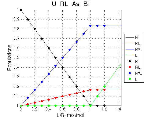
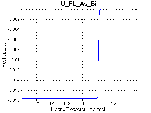
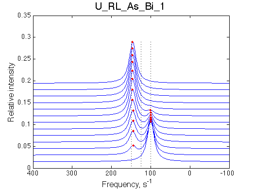
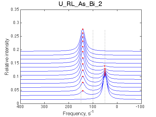
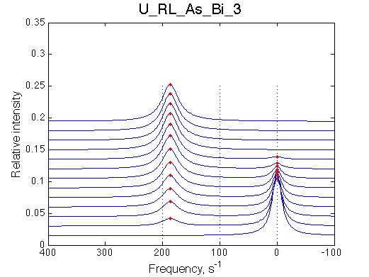
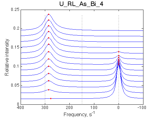
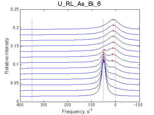
| between peaks/dw(B) | 50/25 | 100/50 | 200/100 | 300/150 | 300/50 | 50/300 |
Simulate setup U_RL_As_Bi_1 |
Simulate setup U_RL_As_Bi_2 |
Simulate setup U_RL_As_Bi_3 |
Simulate setup U_RL_As_Bi_4 |
Simulate setup U_RL_As_Bi_5 |
Simulate setup | |
 |
 |
 |
 |
 |
 |
|
 |
 |
 |
 |
 |
 |
|
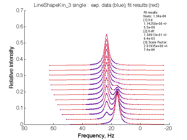
| Optimum norm: 1.34e-04 [1] Kd: 1.14250e-08 +/- 5.5e-09 [2] Koff: 1.38913e-01 +/- 6.4e-03 [3] Scale Factor: 2.01935e+00 +/- 7.4e-04 |
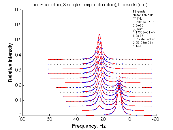
Optimum norm: 1.97e-04 [1] Kd: 1.24050e-07 +/- 2.3e-08 [2] Koff: 1.17300e-01 +/- 8.0e-03 [3] Scale Factor: 2.05128e+00 +/- 1.1e-03 |
Optimum norm: 1.05e-03 [1] Kd: 1.64103e-09 +/- 7.7e-09 [2] Koff: 2.36669e-01 +/- 2.3e-02 [3] Scale Factor: 2.10072e+00 +/- 2.3e-03 |
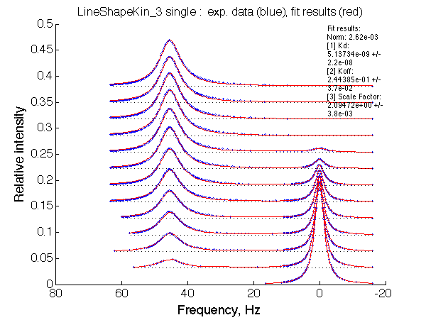
Optimum norm: 2.62e-03 [1] Kd: 5.13734e-09 +/- 2.2e-08 [2] Koff: 2.44385e-01 +/- 3.7e-02 [3] Scale Factor: 2.09472e+00 +/- 3.8e-03 |
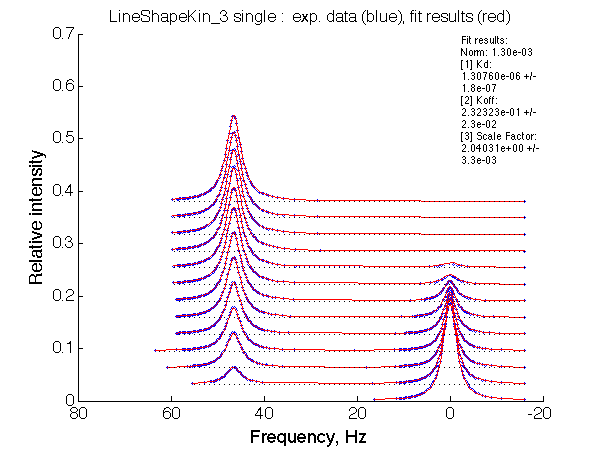
Optimum norm: 1.30e-03 [1] Kd: 1.30760e-06 +/- 1.8e-07 [2] Koff: 2.32323e-01 +/- 2.3e-02 [3] Scale Factor: 2.04031e+00 +/- 3.3e-03 |
Optimum norm: 4.27e-03 [1] Kd: 8.29264e-09 +/- 4.5e-08 [2] Koff: 2.22045e-14 +/- 3.4e-02 [3] Scale Factor: 2.10051e+00 +/- 4.6e-03 |
Conclusion: Tight binding with isomerization of the complex does not leave much trace in the line shapes no matter what chemical shift difference between the end species.
Back to Analysis of Direct and Reverse Titrations