Examples of LineShapeKin applications

This document contains an example of application of LineShapeKin to illustrate features discussed in the Manual.

Contents:

• Examples of different fitting models
  
• References

Examples of different fitting models:
Analysis of titration of RNase A with pTppAp

• Determination of scaling factor for spectral intensities
  (Individual datasets, fixed Kd, variable Koff and Scale Factor)

  ---

• Prelimiary determination of site-specific equilibrium and rate constants
  (Individual datasets, variable Kd and Koff, fixed individual Scale Factors)

  ---

• Determination chemical shifts of titration end point
  (Individual datasets, variable Kd, Koff and w0(B), fixed individual Scale Factors)

  ---

• Final determination of individual equilibrium and rate constants
  (individual datasets, variable Kd and Koff, fixed individual w0(B) and Scale Factors)

  ---

• Determination of global equilibrium and rate constants
  (combined dataset, variable single Kd and Koff, fixed individual w0(B) and Scale Factors)

  ---

• Judging global versus individual binding events hypothesis
  (statistical analysis of fitting results)

  ---

Back to the Top

Determination of scaling factor for spectral intensities
(Individual datasets, fixed Kd, variable Koff and Scale Factor)

First step in data analysis is determination of scaling factor for spectral intensities. Need for scaling factor originates from our practical inablility to include complete lorentzian envelope into the slice. Moreover, individual correction for every set of 1D slices is needed.

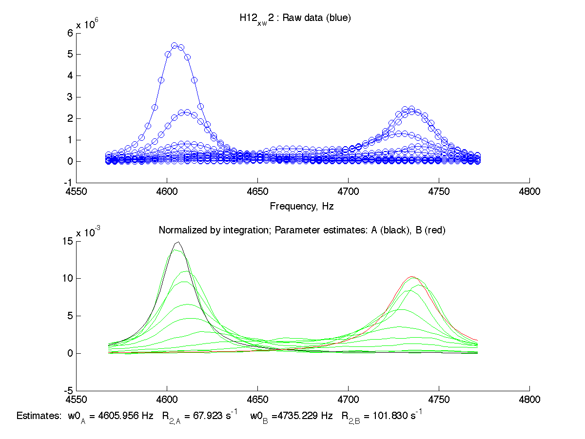
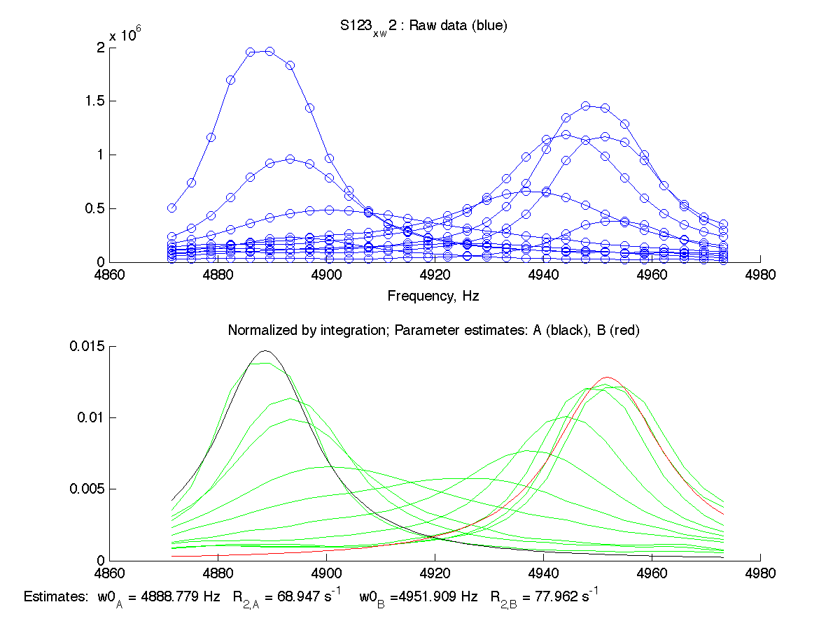
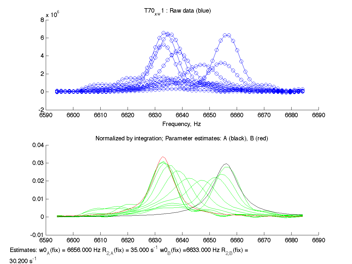
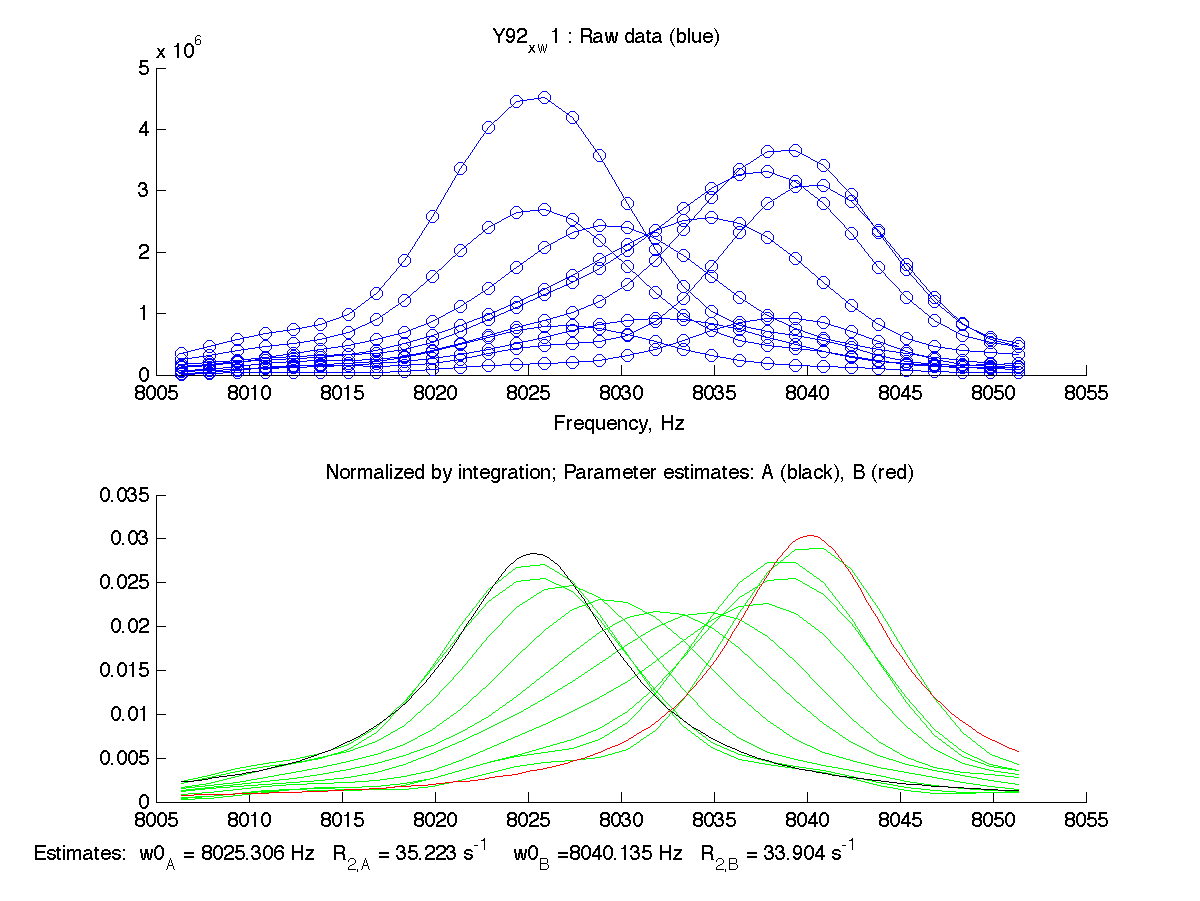
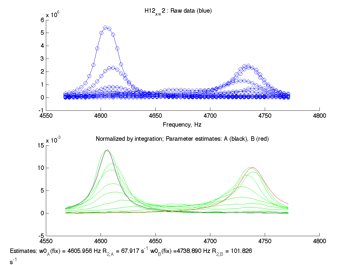
For these for residues below the A and B peak position and relaxation rates estimates generated by 'just display data' mode were good except for T70 resonance. I had to manually adjust R2s and w0 in corresponding files (manual_R2.txt and manual_w0.txt) until black and red traces (states A and B) approximated well the beginning and ending traces of normalized graph (results are printed with (fix) note on the normalization graph) .

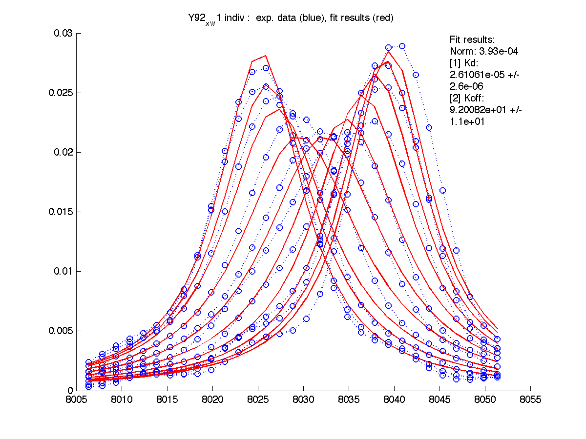
In this work I obtained an estimate of Kd from chemical shift titrations profiles. I fixed Kd=1.4 microM and fitted individual residues (mode 'single'). I took individual scaling factors determined and entered the fitted values of Scale Factor into scale_factor.txt in the peak dataset folders (for every residue separately). Now the data for every residue is scaled using its individual scaling factor upon loading.  I reran fitting to verify that Scale Factor has its value about unity for every peak (mode 'indiv').

The  current folder is 1.Matlab_fitting/.

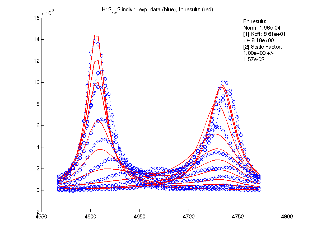
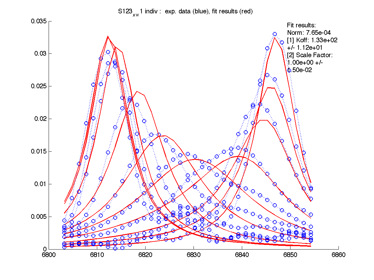
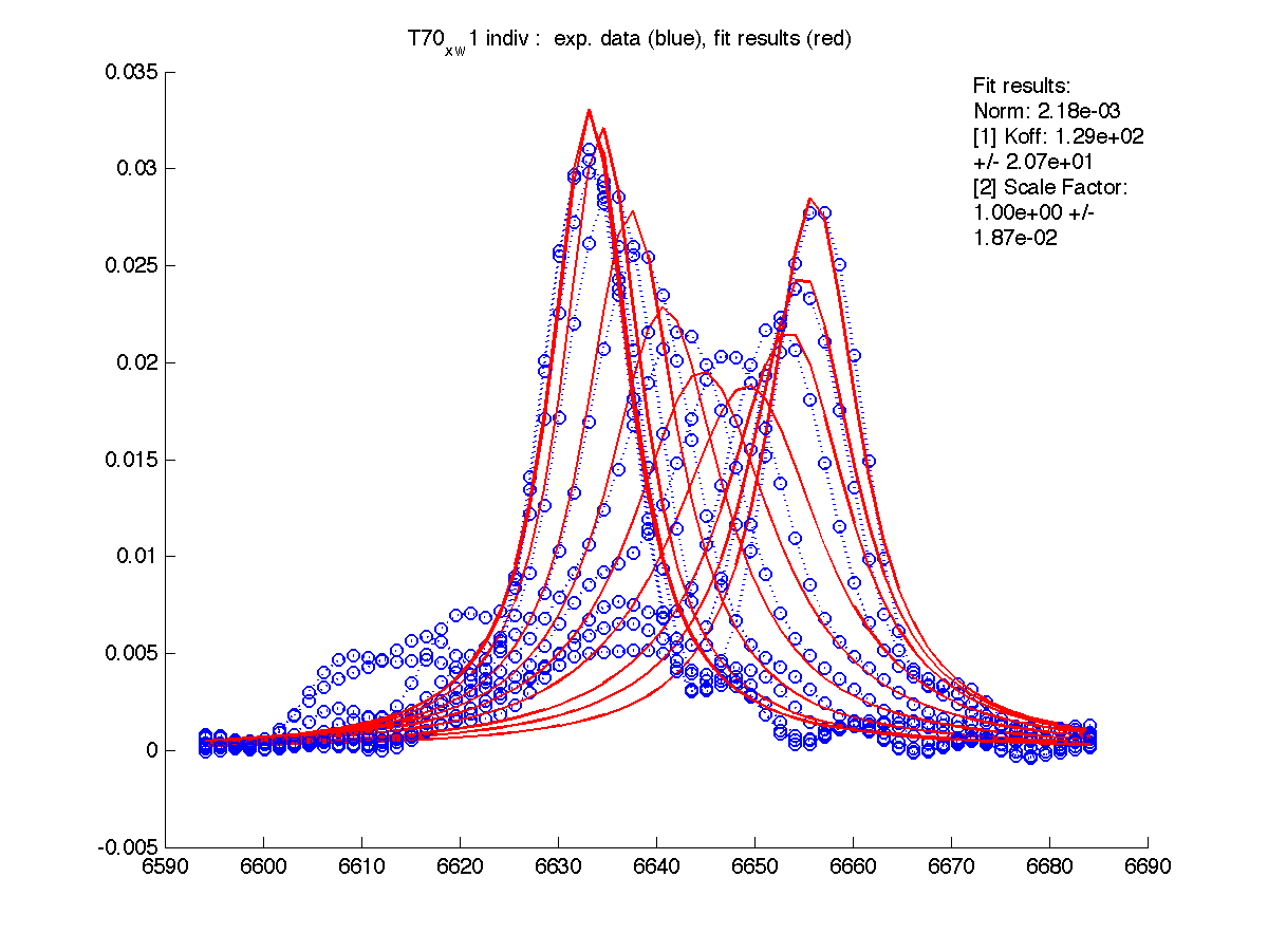
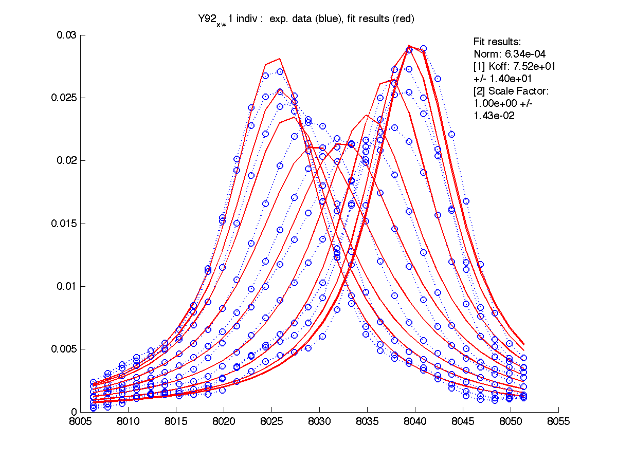
H12, w2	S123, w1	S123, w2	T70, w1	Y92, w1

Back to the Analysis Section

Back to the Top

Prelimiary determination of site-specific equilibrium and rate constants
(Individual datasets, variable Kd, Koff and Scale Factors)

Now we are in a position to fit data as individual residues versus a group fitting. I will alter m-notebooks to add determination of Kd in addition to Koff and Scale Factor.

The  current folder is  2.Matlab_fitting.Koff_Kd_SF.

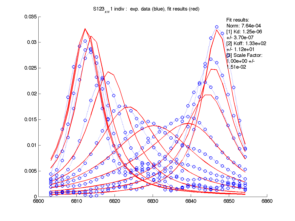
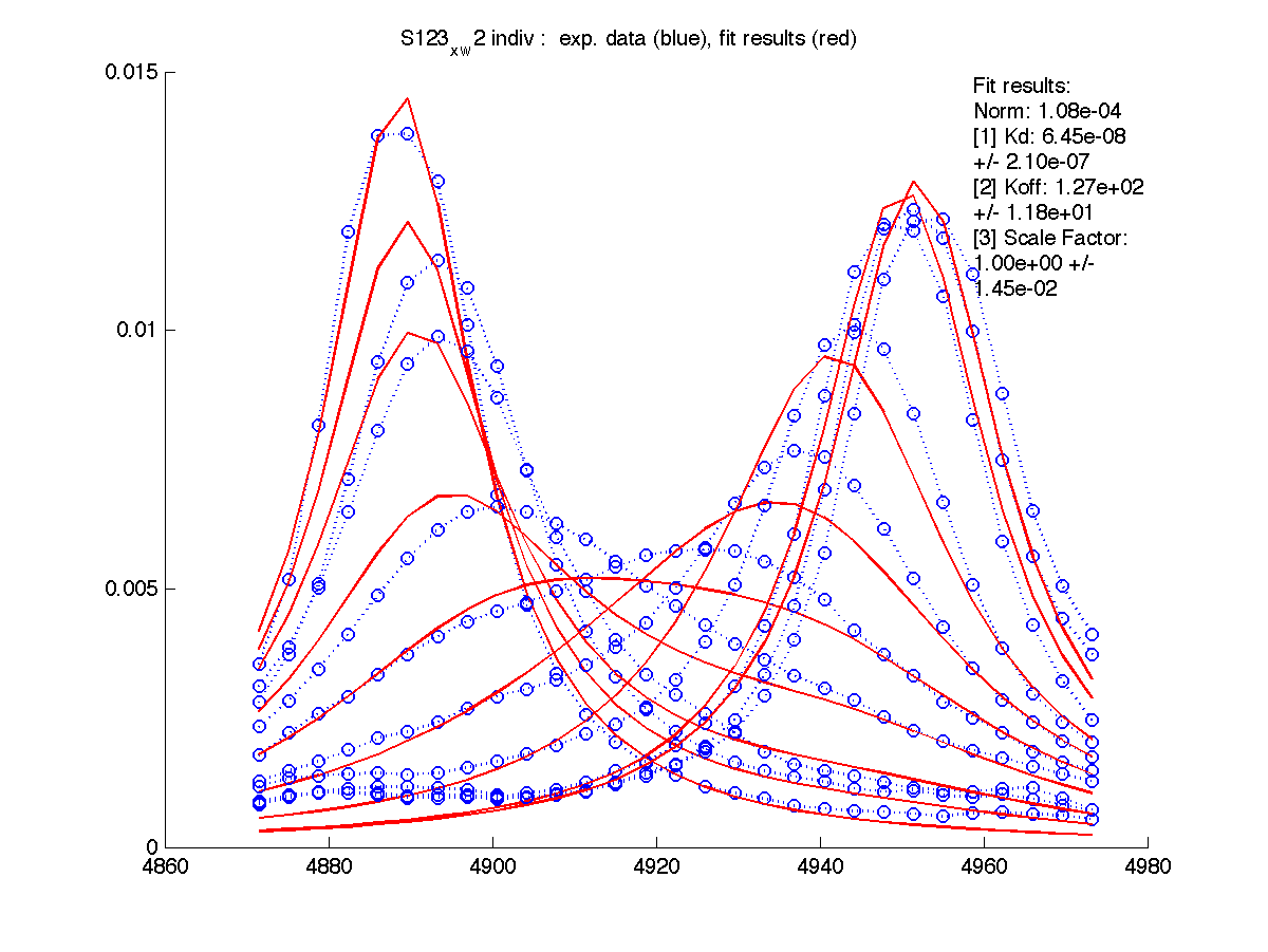
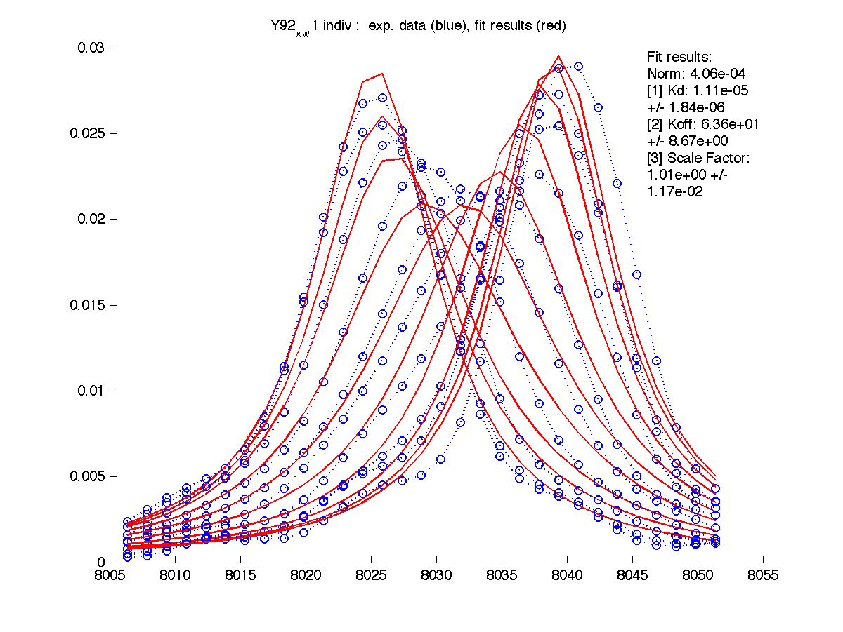
H12, w2	S123, w1	S123, w2	T70, w1	Y92, w1

We can see that Scale Factor is fit to very close to unity. It confirms that the scaling of the raw data is done adequately and we may remove Scale Factor from fitting parameters now.

Let's look at these fitting sessions in comparison:

We see that Kd and Koff are in general agreement with the values from a previous run. Two cases fall out of the line: H12 and T70.

H12 is in slow exchange and Koff and Scale Factor did not change when Kd varied from 1.4 micromolar down to 10^-14. Quality of fitting was not affected by Kd change. This exactly means that for slow-exchangers the line shapes to NOT carry sufficient information for Kd determination. Koff values, however, is relatively reliable.

T70 is an example of a problematic line shape envelope affected by overlap with nearby peaks. Fitting procedure got trapped in  a local minimum with higher Norm value (32e-4 with Kd fitting, while 22e-4 with fixed Kd) trying to accomodate these line shape distortions. Therefore, clean single-peak line shape is a must.

Individual and global fitting of K_d and K_off

Once you determined your Scale Factors and inserted them into scale_factor.txt files, you may go to 3.Matlab_fitting.Koff_Kd.fixed_SF/ and perform K_d , K_off determination utilizing fixed Scale Factor values. This procedure will be faster and will deliver better accuracy of Kd and Koff due to reduction in number of fitting parameters.

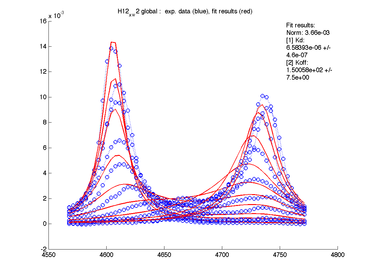
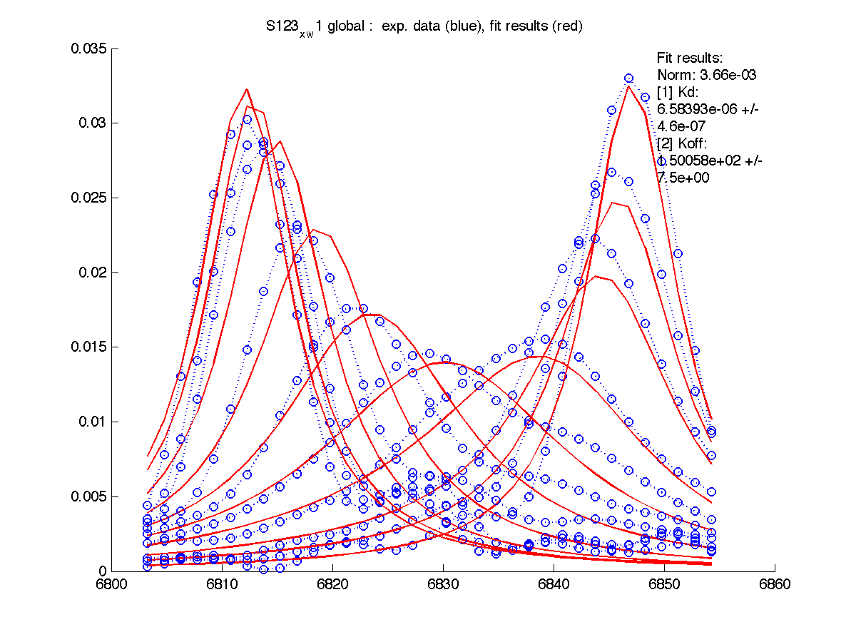
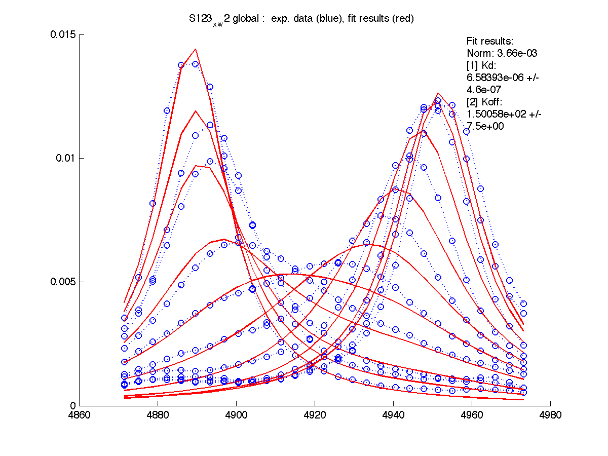
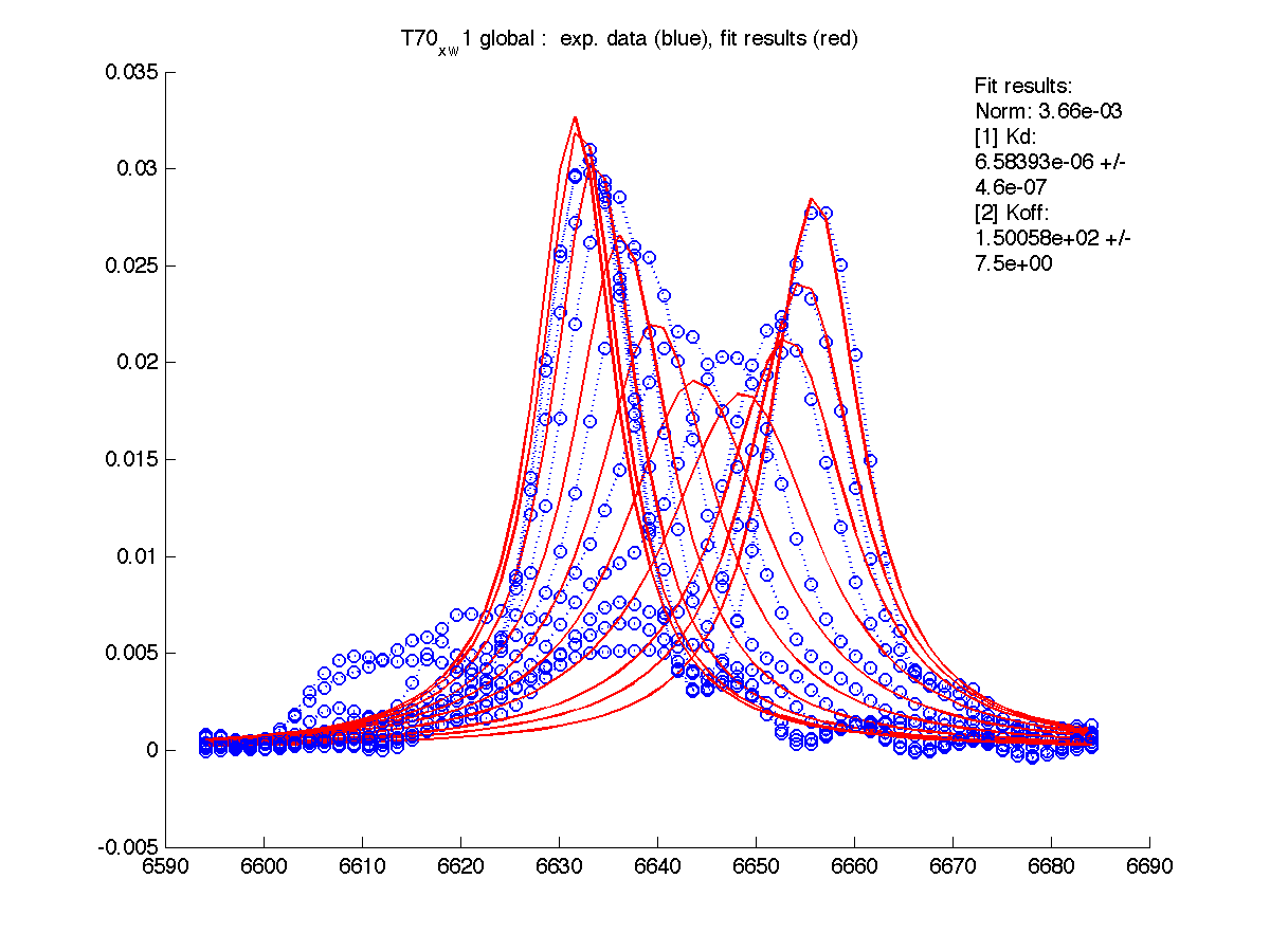
You can do both individual and global fitting of datasets at this stage. The global fitting mode ('global') directs LineShapeKin to construct a composite dataset of all individual sets and fit all this data to a single K_d : K_off combination.

For example of global fitting results see below and statistical testing of global versus individual fitting models below as well as here.

Back to the Analysis Section

Back to the Top

Determination chemical shifts of titration end point
(Individual datasets, variable Kd, Koff and w0(B), fixed individual Scale Factors)

Looking at sources of imperfect fitting we may notice that initial estimates of the start and end of titration are imperfect (see normalization graph above). In many cases, end-point of titration (red trace) does not 'smoothly' follow previous traces and may have been distorted. Another source of a problem is that it is difficult to obtain true estimate of fully formed PL complex if constants are not very tight.  However, because we got rid of one of the fitting parameters now (Scale Factor) we may now easily add frequency of the end-point of titration to a list of fitting parameters and determine it directly.

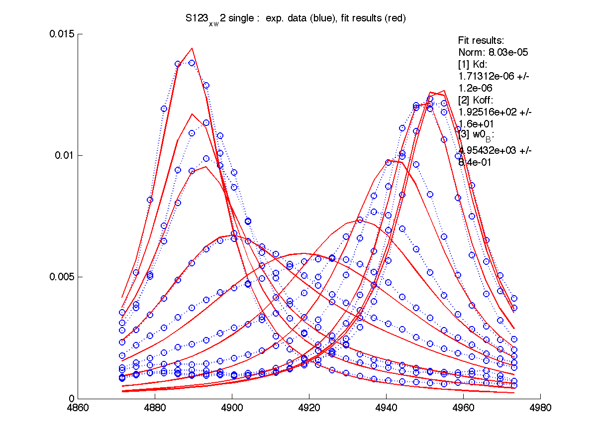
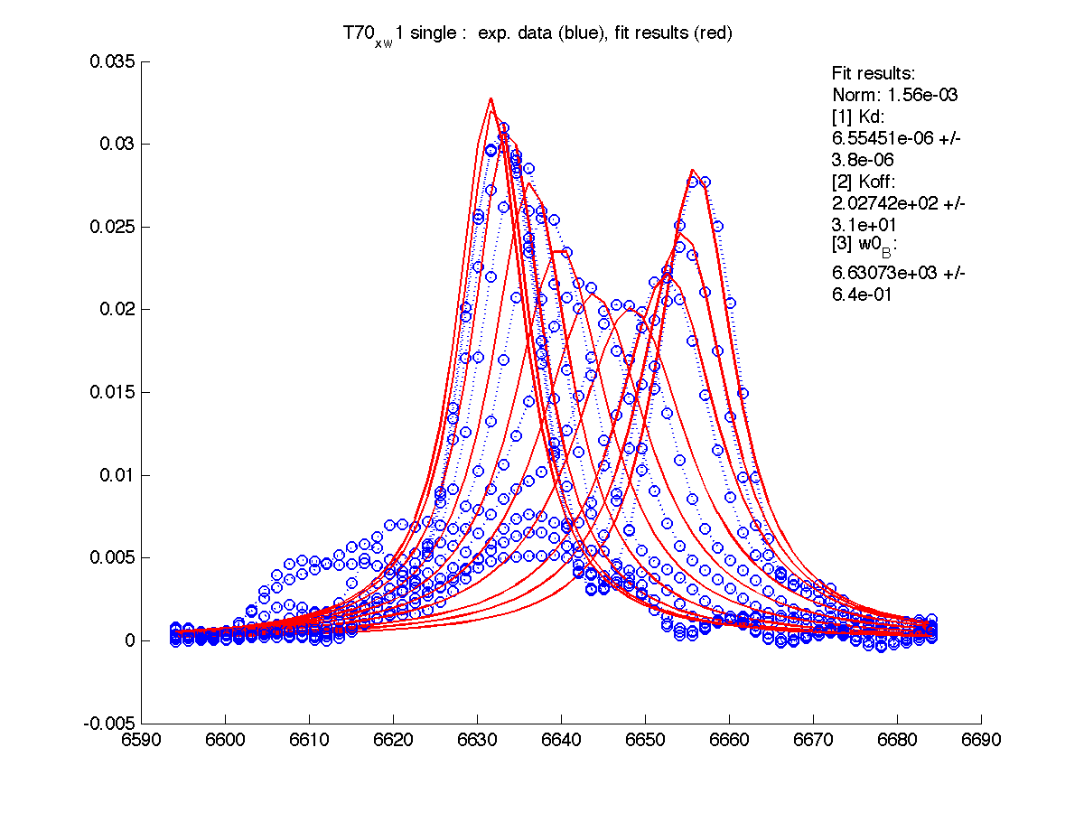
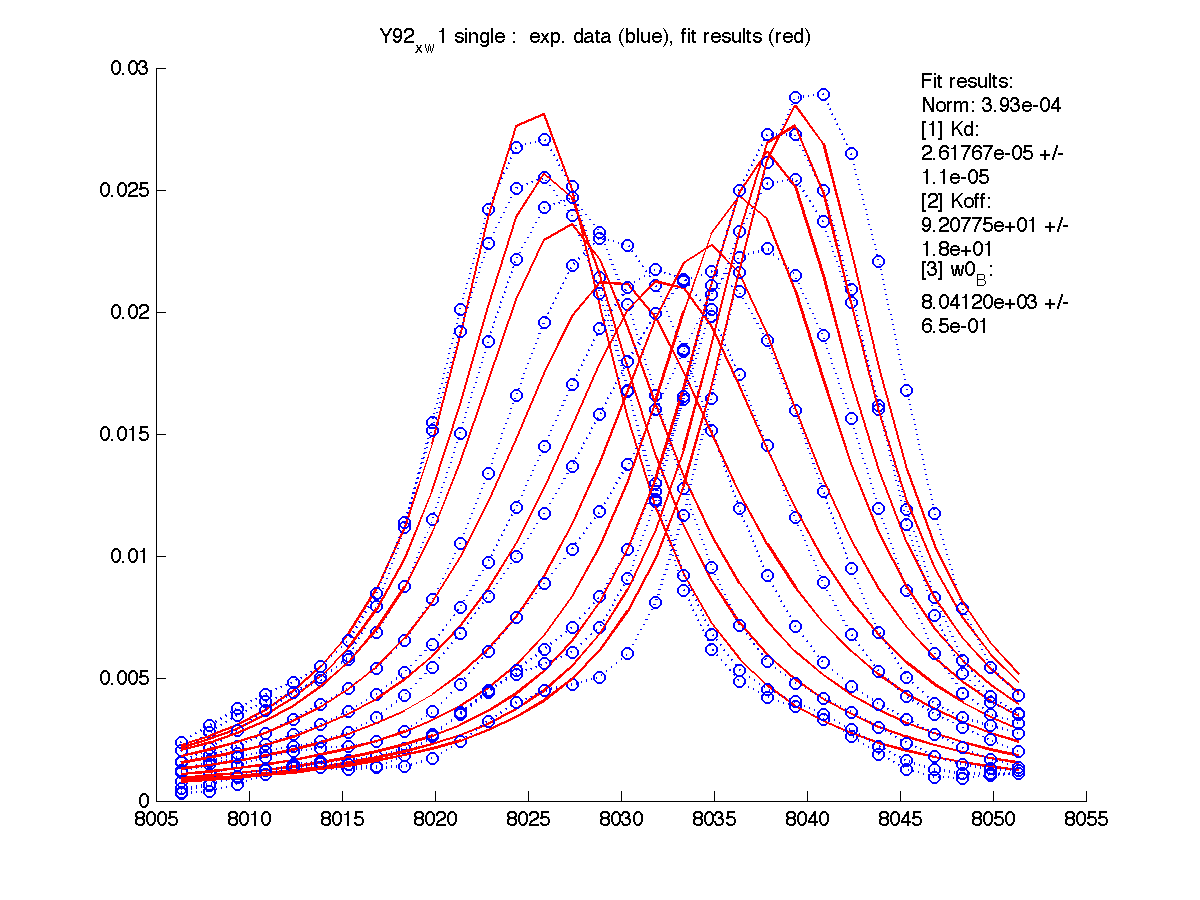
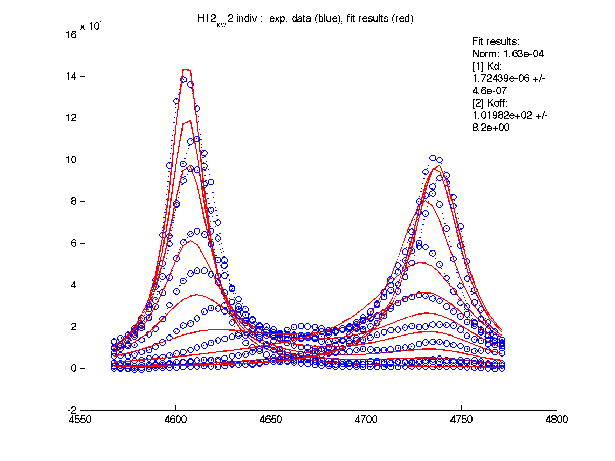
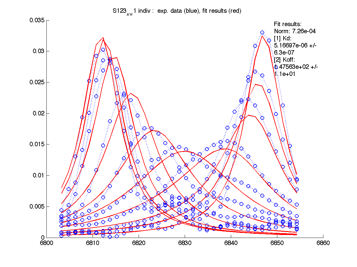
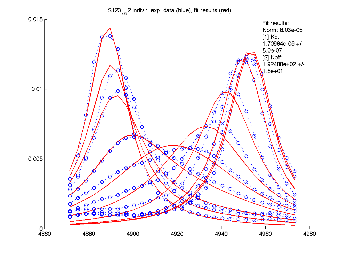
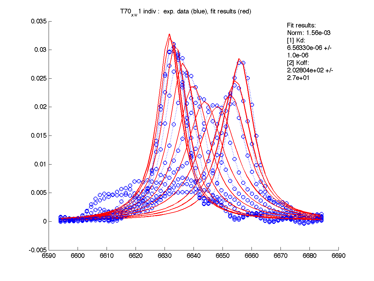
Here we fit residues in the single mode. We enter starting values for w0_B array in setup.m.

The  current folder is 4.Matlab_fitting.Koff_Kd_w0B.fixed_SF.

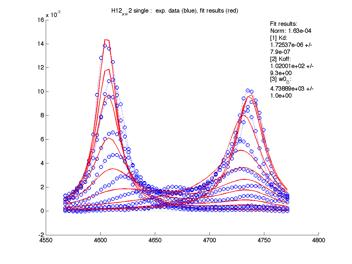
H12, w2	S123, w1	S123, w2	T70, w1	Y92, w1

Now the fitting procedure performs significantly better. Originally failed H12 and T70 fit very well with reasonable estimates for Kd. It means that the last trace was indeed distorted and could not serve as a final peak position for fully bound state B (in addition to slightly incomplete titration profile at L/P ratio 1.3 in the final point).

Back to the Analysis Section

Back to the Top

Final determination of individual equilibrium and rate constants
(individual datasets, variable Kd and Koff, fixed individual w0(B) and Scale Factors)

Fitting frequency of the B state prevents us from running global analysis because every frequency is specific to each residue and current LineShapeKin release does not support fitting both individual and global parameters. To circumvent this problem we will include the frequencies determined above into the files manual_R2.txt and manual_w0.txt in resdue data folders. These files will be read upon data loading and these values will override automatic estimates and serve as constants for data fitting. Now we can remove frequency of state B from fitting parameter list.

To preserve the original data I will copy the Data_for_MatLab/ folder into a local directory and do editing here: 5.Matlab_fitting.Koff_Kd.fixed_w0B.fixed_SF.

Now all frequencies values are reported with (fix) label on a normalization graph signifying that we manually provided the values to use in calculations.

H12, w2	S123, w1	S123, w2	T70, w1	Y92, w1

Normalization graphs show how new peak positions for B state are related to the experimental peaks. As expected, fitting results are identical to previous ones.

Back to the Analysis Section

Back to the Top

Determination of global equilibrium and rate constants
(combined dataset, variable single Kd and Koff, fixed individual w0(B) and Scale Factors)

Now we can hypothesize that Kd and Koff values observed for these four residues are similar enough and may actually represent a response of these residues to a single binding event rather than multiple individual ones.

In order to do this we will switch to global fitting mode ('global') so LineShapeKin will construct a composite datasets of all individual sets and fit all this data to a single Kd : Koff combination.

H12, w2	S123, w1	S123, w2	T70, w1	Y92, w1

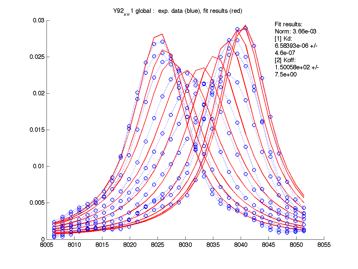Results are saved in grid_results_Y92_x_w1.T70_x_w1.S123_x_w1.S123_x_w2.H12_x_w2.dat

If we compare individual and global fitting graphs now we see that fitting became worse for H12 and Y92 (mainly, because of Koff change to faster values which drove line shapes further toward fast exchange shapes). However, fits are still acceptable overall quality, therefore we may state that these two hypotheses are good but we want to assess rigorously which one is better.

Back to the Analysis Section

Back to the Top

Judging global versus individual binding events hypothesis
(statistical analysis of fitting results)

Here we will use Akaike's information criterion to judge whether a set of individual binding events is more likely than a single binding event reported by multiple nuclei. For more information on Akaike's criterion see [1] and my poster at ICMRBS 2008

I insert residue names into AIC_setup.m from setup.m. I find 'composite' residue name in grid_results_Y92_x_w1.T70_x_w1.S123_x_w1.S123_x_w2.H12_x_w2.dat and insert it as global resname.

Issue compare

Evidence ratio of 260 means global model is 260 times more likely correct than 'individual' in this particular case. In terms of Fisher criterion it corresponds to 99.7% (=100-100/260) % confidence that this data is better described by global hypothesis [1].

The basis for this conclusion is that when we switched 'individual' to 'global' model we reduced number of parameters approximately 4-fold while sum of squared residuals (SS) increased just 50%. Therefore, with the current data for this group peaks it is 260 more likely that we have the global binding event with Kd = 6 microM and Koff=150/s rather than multiple binding events with Kds spread from 1.7 to 26 microM and Koffs from 90 to 200.

Note that this 'global' conclusion is achieved by taking into account number of degrees of freedom together with changes of sum of squares in the fitting procedure. If you look at individual errors reported on fitted values of Kd and Koff - they generally DO NOT overlap. The PRECISION of fitting is indeed this high but ACCURACY of representation of real situation has to be judged by statistical means.

Current conclusion of precedence of global hypothesis does only mean that the current data set of 4 residues in RNase A DOES NOT SUPPORT hypothesis of local binding events. In other words, quality of fitting of individual residues using individual equilibrium and rate constants is not so much better to warrant consideration of these additional parameters. Additional data may improve certainty of this conclusion or lead to a different one. However, based on current result it is 260 times more likely that if we add more residues to a test, the data will support global hypothesis.

Back to the Analysis Section

Back to the Top

References

1.            Motulsky, H. and Christopoulos, A., Fitting Models to Biological Data Using Linear and Nonlinear Regression: A Practical Guide to Curve Fitting. 1 edition ed. 2004: Oxford University Press, USA. 352 PDF version

Back to the Top