Statistical analysis in LineShapeKin

Statistical comparison of individual and global fitting results

If changes you observe in NMR spectra are related to a single binding event than all the residues should display comparable kinetics. Indeed if you do individual fitting you may see similar k_off for a group of residues. You need to apply statistical testing in order find out which hypothesis is more likely: single K_d, k_off for all residues or individual for each. In fact, from statistical point of view it is individual hypothesis that is to be examined because it has increased number of parameters compared to global (single K_d, k_off ). Global hypothesis is simplest and is null hypothesis from the statistical point of view.

NOTE: Here you may only test models that use all their parameters as global. For example three-parameter model Kd-Koff-w0B will not work because w0B is individual for each data set. You can go around it though inserting w0B into manual_w0.txt for each residue and switch back to Kd-Koff model. If you need to compare which model in a sense of different parameters kept constant or variable is more correct when applied to the same dataset see below

To do statistical testing LineShapeKin uses Akaike's Information Theory. In order to perform testing of global versus individual fitting modes:

you should select a list of residues you want to test and put it into setup.m.
run both individual and global fittings.
(resname_x_w?_SS.txt files are generated for each fitting containing number of titration points for each residue and a sum of squares )
IMPORTANT: Before running global fitting and hypothesis testing you must insert Scale Factor values determined in individual run and RE-RUN individual fitting so sums of squares are computed with new scaling factor now!
edit AIC_setup.m to insert the same residue list into its resnames variable.
Look up a composite residue name corresponding to the global fitting results from grid_results_...long-composite-name...dat. and insert it into global_resname variable of compare.m
issue compare on a Matlab command line
the results are displayed on a screen and saved in a text file. For the interpreation of Akaike's test resutls Examples .
If you like use Fisher test use Sums of Squares (SS), N (number of data points) and K (number of parameters +1) to calculate Fisher statistics yourself.

Back to the Contents

Determining the likelihood of different models

In previous section we were discussing application of the same mathematical model to either each residue-specific dataset individually or to a combined dataset of spectral data from all residues. Different task is when you need to decide whether to go with 1, 2 , 3 etc. - parameter models for the experimental data sets.

When you switch the models to fit the same data set you need to determine which model is more likely to be correct. Most certainly the model with larger number of fitting parameters will produce lower norm from fitting. However, one needs to determine whether this reduction in sum of squared residuals is more than statistically expected from a larger number of parameters. If it is more then expected then the model is better describing the data because extra parameter help to take into account some specific feature. Otherwise you should stay with the simpler model.

Example 1: Adding variable frequency of the bound state

In some cases we may think that our titration was not finished and the final spectrum does not represent the chemical shifts of pure state B. In this case we can use a model with variable w0(B) that compensates for incomplete titration.

We fit data in 'single' mode use 2-parameter and 3-parameter models

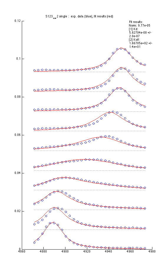
Mode 1: Kd and Koff	Model 2 : Kd, Koff and w0(B)

Using variable w0(B) reduces sum of squares 20% but is it enough to warrant fitting three parameters?

We will run analysis of the two fitting results in terms of Akaike's Information Criterion here:

Adjust paths and number of parameters in AIC_setup_2models.m
Issue compare_2models

Model_1.vs.Model_2.txt contains:

Performing evaluation of likelyhood for each model by Akaike's Information Criterion
1st Model
N = 10
K=3
SS = 9.77181e-05
AICc=-105.36
2nd Model
N = 10
K=4
SS = 8.03361e-05
AICc=-101.319
Model 1 is more correct
Evidence ratio (model 1 is more likely than model 2 by factor of): 7.5e+00

Interpretation:
- Evidence ratio tells us that the model with 2 fitting parameters (model 1, variable Kd and koff) is 7 times more likely to be correct than the model with additional variable chemical shift of a B state.
- However, scientifically, the three parameter model worked better than two parameter as it reproduced experimentally detemined micromolar Kd, in contrast to nanomolar Kd obtained in 2-parameter fitting. However, in both cases Kd is barely statistically significant or insignificant, so this argument is weak.
Conclusion: we should keep testing both models on our data.

Example 2 : Adding correction for concentrations.

LPcorrection/

Here I tested whether the extra parameter for correction of L/P ratio is needed in the fitting procedure (to compensate for imprecise concentrations in the titration series).
- 3-parameter model (Kd, Koff and w0B) was fitted here for two residues individually
- 4-parameter model (+L/P correction ) was fitted to the same data here
I am computing Akaike's Information Criterion test for these two models here . The model with lower AICc will be more correct. Evidence ratio tells us how much more likely correct.
- I entered folder names for the two model fitting results and number of parameter in each model.
- I do testing for each residue individually.
Results revealed that simpler 3-parameter model is 40-60 times more likely than 4-parameter one (see output) so we can draw a strong conclusion in favor of simpler model 1.
Conclusion: Concentrations of chemicals were correct in my experiments and correction for concentration is NOT necessary (not supported by the data).

Back to the Contents