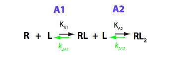
The model where two ligand molecules bind to one receptor molecule is termed B in the current analysis. Binding involves two steps with one ligand molecule binding at a time. Convention in what follows is that all the equilibrium constants are the association constants (shown in black below) and kinetic constants - reverse (off-rate) constants (in green). I have graphically analyzed B model in B_model.pdf
This above scheme is the simplest description of the binding process done in terms of macroscopic constants. However, molecular-level interpretation is more straightforward with the more detailed scheme of binding reaction making use of microscopic constants (Cantor and Schimmel 1980). Microscopic constants do not include statistical contribution and may be interpreted in terms of individual interaction energies.
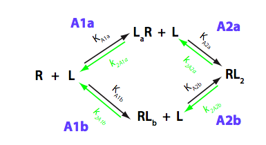
We should consider that R has two binding sites, in general case - unequal in binding affinity to L. Additionally, binding of a second L molecule may have lower or higher affinity due to negative or positive cooperativity between the two binding sites. Microscopic constants allow direct evaluation of allosteric effects between the sites so we will perform all analysis in microscopic terms. The modified reaction scheme is given below.
Relationships between the micro- and macroscopic equilibrium constants in two schemes are as follows:
![]()
In case of identical binding sites the microscopic constants on parallel paths are equal
![]()
![]()
![]()
![]()
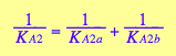
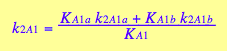
and macroscopic constants are related to them as
![]()
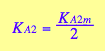
Further, if we assume no interaction between the two sites, then KA1m =KA2m, which results in the relationship between the first and second macroscopic binding constants:
![]()
This is a purely entropic, statistical factor of increasing the number of species in the first binding and decreasing the number of species in the second binding event which makes the second macroscopic constants four times weaker even if molecular binding event produces the same free energy change no matter whether the second site is free or occupied (microscopic binding constants are equal). See more discussion on microscopic and macroscopic constants in (Cantor and Schimmel 1980) or any other physical chemistry text.
Kinetic constants are also related as follows:
![]()
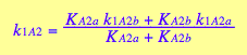
![]()
If the two sites are identical then
![]()
![]()
![]()
![]()
Further, if there is no interaction between the two sites then the microscopic constants in the following steps are equal and that relates macroscopic constant of the two step as follows:
![]()
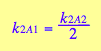
In other words, due to statistical effect of diverging alternative pathways in the A1 step the macroscopic forward rate constant appears twice as large relatively to A2 step. Reverse rates are connected in reciprocal fashion: divergence of reverse pathways in A2 makes reverse rate constant in A1 appear twice as slow relatively to A2 if considered macroscopically.
Obviously, macroscopic consideration mixes statistical factors into both equilibrium and kinetic rate constants thus making molecular interpretation of those quantities more complicated. Therefore, in the analysis of B model I utilize microscopic constants.
Important note on differences in labeling of transitions and binding sites: The labels 'a' and 'b' were chosen to assign microscopic equilibrium and kinetic constants to the two pathways in this model, NOT to label binding to the two distinct binding sites, I and II. If we assing binding of the ligand molecule to the site I in unbound R with the empty site II to the transition A1a, it is followed by binding of the ligand molecule to the site II in A2a. However, binding of the ligand to the site II, when the site I is empty, occurs in transition A1b, followed by binding to the site I in A2b. This is important to keep in mind when interpreting numeric values of the microscopic binding constants.
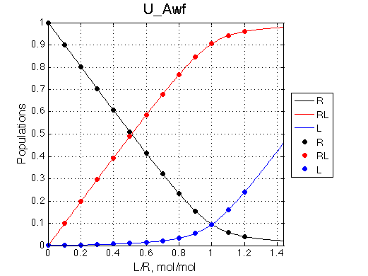
Analyzing every complex model we should be able to predictably reduce it to a simpler one. B model is extension of U model by adding one more binding site. Let's see if we can reduce B to U and reproduce results of one of the U test cases.
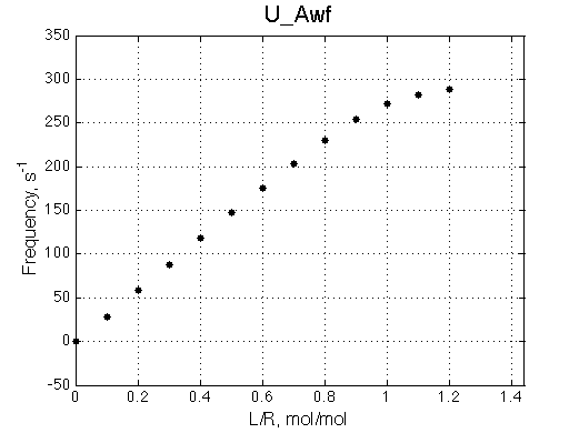
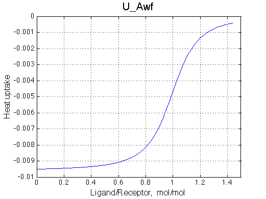
A 'target' U model will have Ka=1e5 and k2=1000/s (U_Awf.txt in U ).
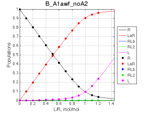
We want to remove A1b, A2a and A2b transitions by setting corresponding k2 =0 and K=1e-3 (B_A1awf_noA2.txt).
Issue Simulate setup B_A1awf_noA2
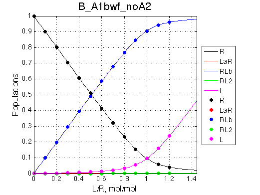
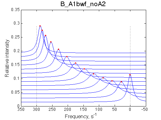
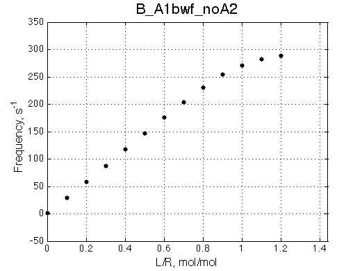
Second test is to turn off A1a and use A1b transition instead (B_A1bwf_noA2.txt).
Issue Simulate setup B_A1bwf_noA2
Results are compiled in summary_report
Here is comparison table of the results:
Simple 1-1 binding |
Two-site model with only A1a transition operative |
Two-site model with only A1b transition operative |
 |
 |
 |
 |
 |
 |
 |
 |
 |
 |
 |
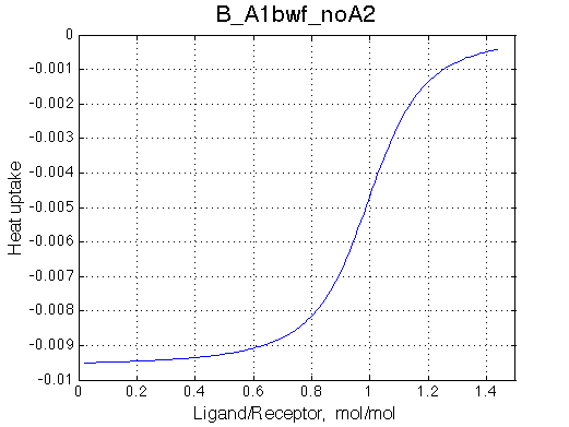 |
All three results are indistinguishable from each other confirming symmetry of equations derived for the model analysis. Further confirmation that the model works as expected is derived in the next sections.
Back to Analysis of limiting cases
Here we will
Below is the summary table (pulled from summary_report)
Site #1 having better affinity for L |
Site #2 having better affinity for L |
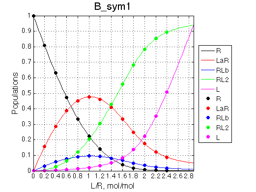
| Issue Simulate setup2 B_sym1 | Issue Simulate setup2 B_sym2 |
 |
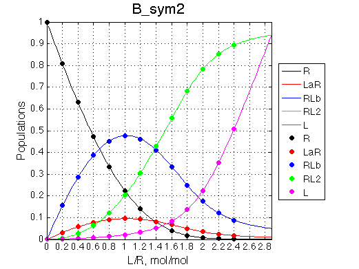 |
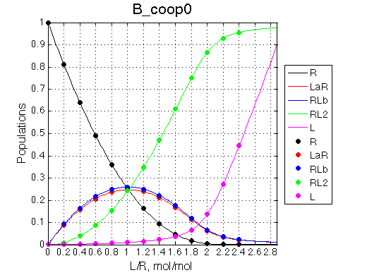
Populations graphs demonstrate that we indeed are able to invert populations of single-bound species by exchanging the binding constants of the two sites.
|
|
 |
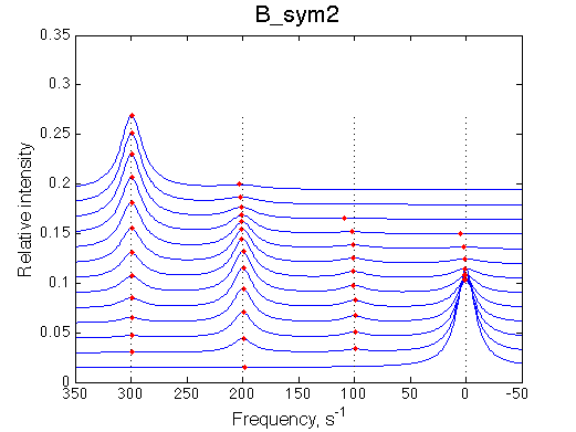 |
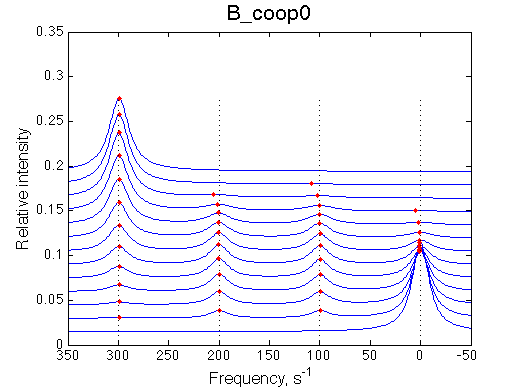
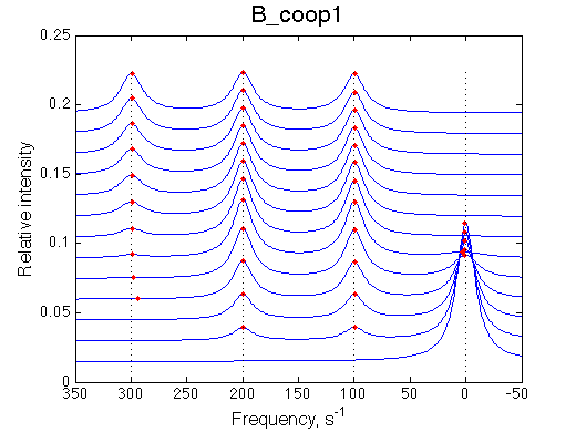
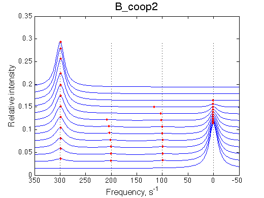
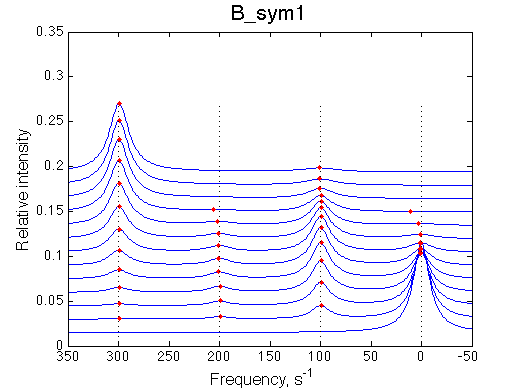
Depending on which single-bound species is more populated we see appearing-disappearing peak at that position, while the other is very small.
|
|
 |
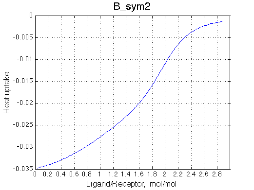 |
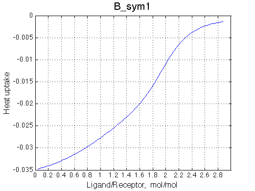
Calorimetric curves are identical because I exchanged the heat effects of formation of the single-bound species as well. The heat release is large in the beginning due to rapid accumulation of the RL forms. However, when the final RL2 complex forms, it leads to reduction in the concentration of the RL species which 'eats up' heat effect of transition therefore the curve looks less sigmoidal.
|
|
Back to Analysis of limiting cases
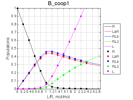
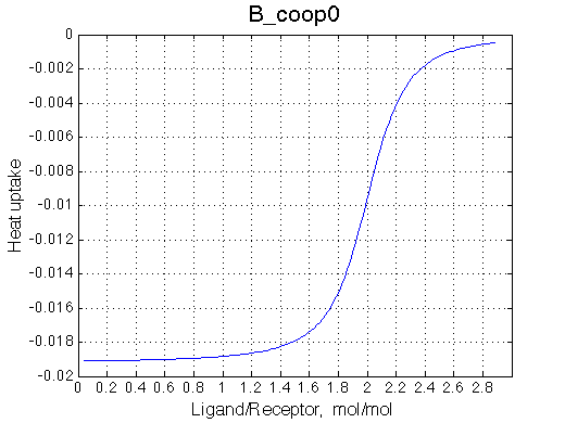
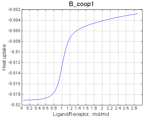
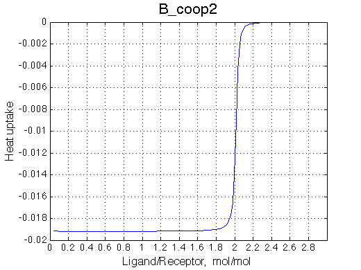
Here we will explore possible interaction of the two binding sites. We will make them identical and have them bind the ligand weaker if the other site is occupied (B_coop1.txt), which is negative cooperativity, or tighter (B_coop2.txt), which is positive cooperativity (I also made binding constants on paths 'a' and 'b' 5% different to avoid complete overlap of curves for single-bound species on population graphs for easy viewing).We will utilize setup3.txt to direct simulation output into a different folder Example_simulation_cooperativity/.
Summary report is summary_report and I lay out graphs side by side below:
Back to Analysis of limiting cases
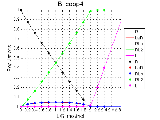
The positive and negative cooperativity of binding sites may be explained by either direct (electrostatic, steric, etc) or indirect (allosteric) interaction between binding sites. Let's assume a positive cooperativity with additional enthalpy change due to interaction with occupied neighboring binding site (on top of enthalpy due to interaction with the own binding site). The populations for positive cooperativity are as follows:
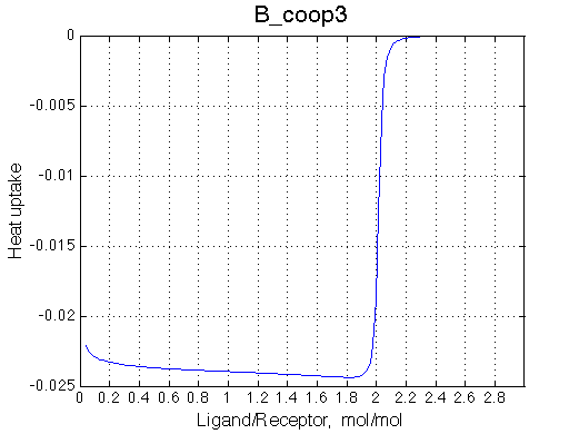
>> Simulate setup3 B_coop3 # Heat of formation of the species, relative units |
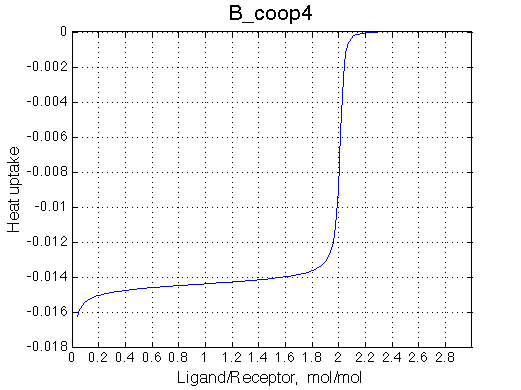
>> Simulate setup3 B_coop4 # Heat of formation of the species, relative units |
 |
 |
The pre-transition profile is distorted. The binding heat of binding is smaller until formation of RL2 becomes strongly preferred thus releasing both binding and interaction enthalpies.
|
The pre-transition profile is distorted The beginning of the curve has larger heat because relatively less of RL2 species are formed and the very beginning. Once L concentration increases, RL2 becomes strongly preferred and binding heat decreases due to opposing enthalpy of cooperative interaction between sites. |
B model works as expected.
Back to Analysis of limiting cases
Cantor, C.R., and Schimmel, P.R. 1980. Biophysical Chemistry. Part III. The behavior of biological macromolecules. W.H. Freeman and Co, New York, pp. 360.
Cavanaugh, J., Fairbrother, W.J., Palmer III, A.G., and Skelton, N.J. 2006. Protein NMR Spectroscopy: Principles and Practice. Academic Press, pp. 587.
Back to LineShapeKin Simulation Tutorial