Setting up simulation in LineShapeKin Simulation is a simple linear process. In this document I will go through some of the installed models doing example simulations.
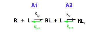
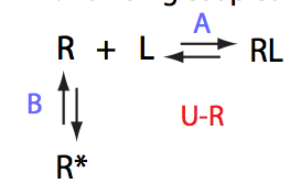
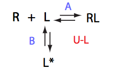
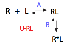
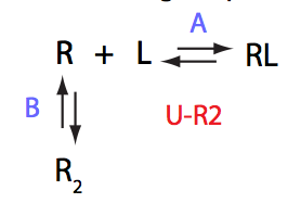
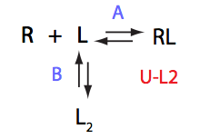
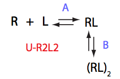
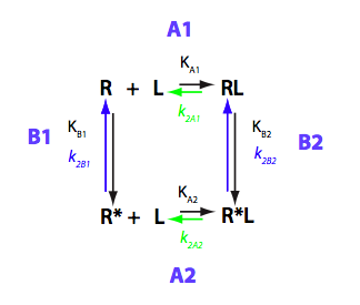
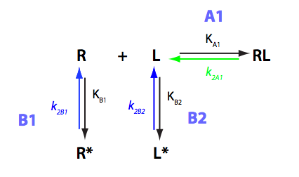
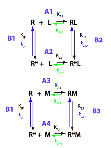
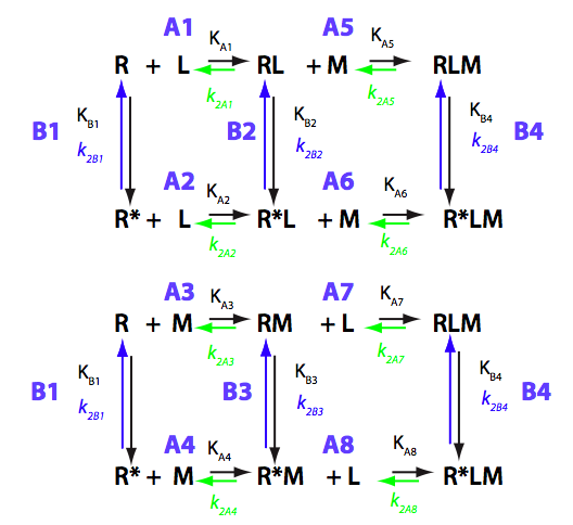
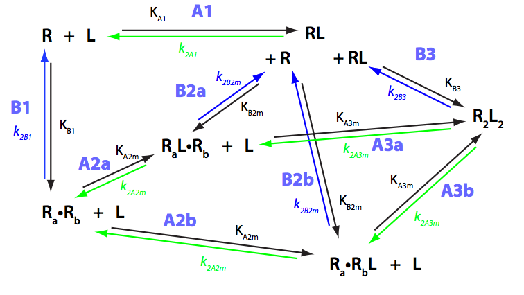
Schematic representation of all the models may be found in Models/. All models are labeled with the code that helps to uniquely identify them. These codes are not based on any rigorous nomenclature instead only serve as nicknames generated using simple rules. The code contains U if only one molecule of ligand binds to a receptor or receptor dimer. B stands for two-site binding. Whenever isomerization of some receptor-ligand complex occurs, this form is included in the code (ie RL). If any receptor-ligand complex dimerizes it is included as R2 or R2L2. This coding convention only serves purpose of distinguishing between the models.
The MuPAD notebooks with derivations of the equations for these models are available upon request.
The simulations involve numeric solution of the equilibrium thermodynamics equations and may become unstable if the binding constants of very small magnitude are involved. This may be the case if you intend to turn off some of the model pathways and set binding constants to something like 10-16. While generally that does not cause any problem in simple models, if you set the subsequent constants to 10-16 their multiple will become 10-32 leading to rounding errors. Therefore, it is advisable to use formation/association constants for species you want to remove from the mechanism on the order of 10-6. Such formation or association constants lead to tiny populations of species in the practical range of the receptor concentrations and will not cause instability of numeric solutions.
A good practice is to examine values of dependent constants calculated by the program in the output. If some become too large or too small you should tweak constants on the pathway to keep the meaningful ratios between the species but reduce their overall magnitude.
It is mandatory to perform a reality check of the computation results: all calculation results must comply with common sense and show expected features when their parameters are varied. It is useful to examine the complex models by (1) reducing them to the corresponding simpler models, and (2) simulating verifiable limiting cases to test performance of the algorithm and build some intuition for the complex model behavior. If you observe something that looks like a simulation artifact, please, email me at
![]() .
.
Basic features of the package and a workflow for model parameter setting is described in discussion of the U model below
One of the examples of analysis of complex line shapes originating from exchange between multiple species may be found in description of the U-R-RL-RM model
NOTE: All the models are analyzed in the folder: LineShapeKin_Simulation_4.1/tutorial_simulations/. This is your source of the example setup files for any models.

