
This is the most generic binding model. I will utilize it to highlight the features of the LineShapeKin Simulation as well as to demonstrate curious experimental outcomes originating from this ever simplest binding mechanism.

A folder U/ contains the following:
General settings for the simulation (model-independent) are set in a file setup.txt. You may choose any different name and you may have multiple setup files with different design of experimental series and output settings. Extension TXT is required.
Simulation results will be placed into a local folder set by Results_Path. If you want to run simulation for the same model but different general settings while keeping your previous results - change this variable.
I include some titration points for my simulation of NMR line shapes in the field LRratio, which is a molar ratio of total ligand to total receptor concentration in the sample. Note that the first point, corresponding to L/R=0, must be set as small positive value (to avoid division by zero).
Populations of species and ITC profiles will be computed using more points (to make curves smooth) set by LRpoints. Computation of populations is most time-consuming task so with the complex models we may want to reduce this number.
The complex models including two different ligands, L and M, will make use of MRratio - a total M to total R molar ratio, while in the models without M this field is ignored.
Total concentration of the receptor, Rtotal, is set for every LRratio point. For simple analysis I keep it constant. However, you may vary it to simulate your experimental conditions. Note, that smooth curves will be still computed for fixed Rtotal in this version.
Display of the NMR line shape simulations is controlled by Spectral_Points, w_min and w_max fields, which set number of points in the 1D trace, minimum and maximum frequency (s-1 ) of the spectral window, correspondingly.
Overlayed vs. stacked 1D trace representation is set by Stacked_Plot (YES or NO) with a vertical displacement of every next trace in stacked representation by a percentage of the peak height set by Percent_Shift.
Multiple model setup files may be created to explore different possibilities. First, I will make a file U_Awf.txt to simulate 1:1 binding (so I put U and A in the file name), relatively weak (so w) and fast off-rate (f). You may use any file names you like as long as there are NO spaces. This name will become a label on all graphs and the file names.
First, I am telling LineShapeKin what model to use in Model_code field.
Description may contain any descriptive string for this parameter set.
Association/formation constants are named by a transition name. Transition names are inserted in Ka_names and Ka values in Ka. Note, that not all transitions will be listed here as for any complete cycle of, say, four transitions we will have only three independent equilibrium constants.
Rate constants are also labeled by a transition in k_names and set for every transition in k2 field. Note, we utilize here reverse rate constants in units s-1.
Names of species containing R go into Species_names. The order of these names sets the order for values in R2, and w0 fields, setting base transverse relaxation rate of pure species and their chemical shifts (in units s-1 ).
Isothermal titration calorimetric profile is simulated using specific heats of formation of the species set in dH. We define the initial receptor form as a standard state with dH=0 and any other state measures its formation enthalpy relatively to this initial standard state (not to a previous reaction step in multistep mechanisms).
All ready to go. Issue Simulate setup U_Awf. (Note: you don't need .txt extension here.)
Graphic windows pop up on a screen as they are generated, saved on a disk and assembled in an HTML report summary_report.htm viewable in any web browser. This document compiles images created by LineShapeKin Simulation in a convenient format. All the graphic files are located in Example_simulation/U_Awf/ (as set by Results_Path variable and the model setup file name U_Awf). Title of the model section in this report U_Awf links to this folder.
Example simulation results are shown below:
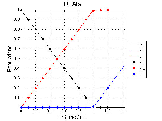
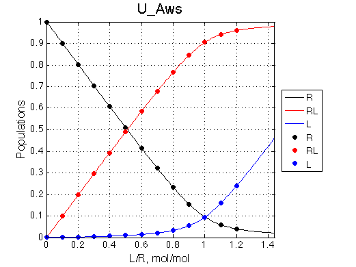
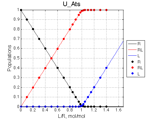
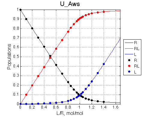
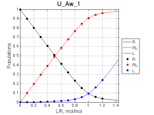
Populations of all species are calculated for the requested L/R points as well as in a form of a smooth curve extending 20% beyond the L/R range. Populations of multimeric species are shown per monomer. Population of free ligand is normalized to total receptor concentration. |
 |
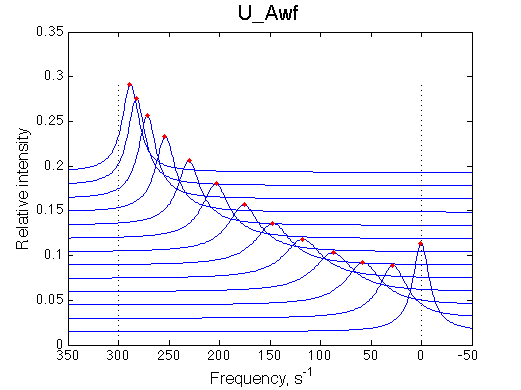
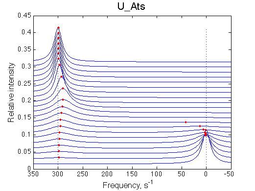
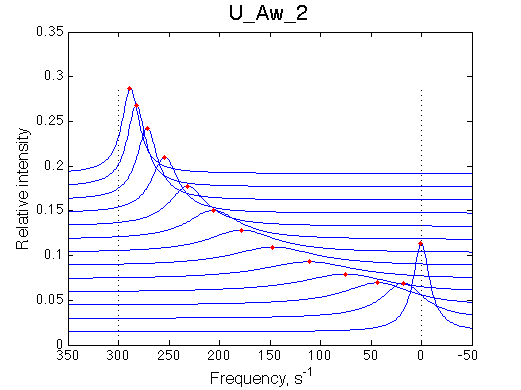
1D traces (from bottom to top) correspond to L/R ratios indicated by points in the Populations graph (LRratio values). Red dots indicate peak maxima for a visual aid (also plotted as the chemical shift titration curves on the right). Dashed lines indicate chemical shifts of individual species. |
 |
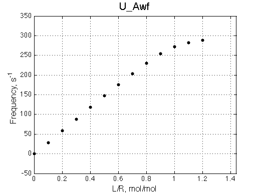
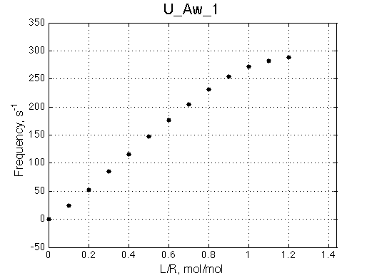
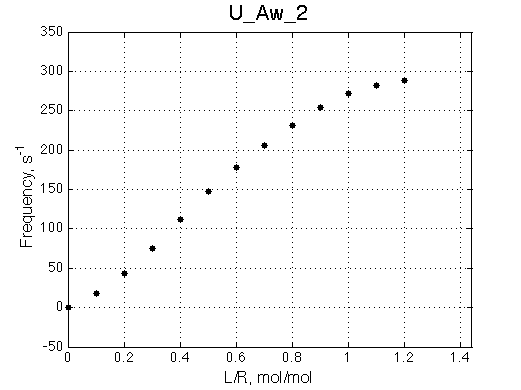
Chemical shift titration curve. This graph may be a quite misleading representation of a titration progress as shown in the next section. However, since this graph is frequently analyzed in NMR titration studies it is useful instruction tool. Points correspond to positions of peak maxima numerically detected in the spectral traces. Sometimes peaks that are detected will not be observed if real signal/noise ratio is considered. |
 |
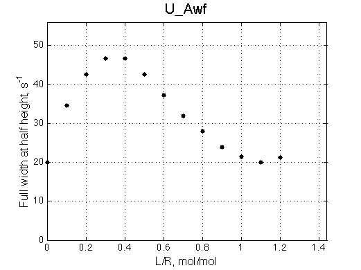
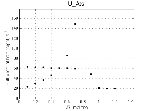
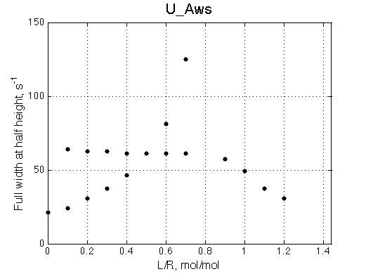
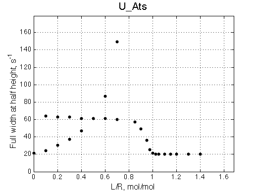
A line width plot is created for all the peaks found in the spectrum to provide another view of the model's behavior. For lorentzian line shape the full-width at a half-height (FWHH) is equal to 2*R2. The FWHH is determined numerically, so sometimes the measurement fails for some points. However, plain-text format data file is saved so you may manually correct and re-plot in any plotting program. |
 |
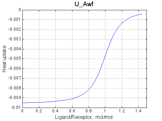
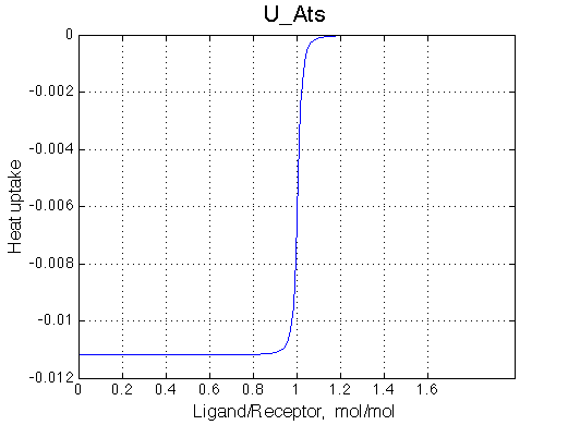
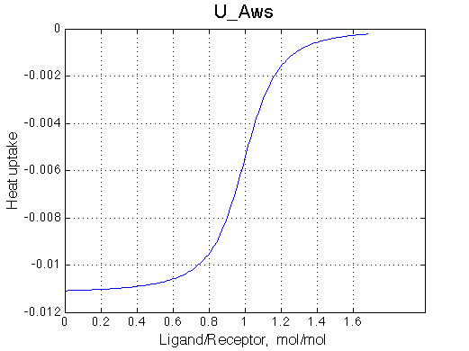
ITC profile simulation is meant to show you what you may expect in your system in ITC instrument. However, normally concentration range for ITC experiments is different from concentration range in NMR so curvature of the real ITC profile will be different. To simulate real ITC profiles all you need is to change Rtotal as dictated by c-value to be in a range of 1-1000 (c=Ka*Rtotal*N, where N is stoichiometry of binding, here N=1). The Rtotal is appropriate for ITC of U_Aw models (c=200) and too high for U_At (c=10000) so Rtotal needs to be >10-100 lower for accurate ITC measurements. Heat uptake curve is simulated as a derivative of the population of species multiplied by specific dH. Dilution of receptor is not considered in the current implementation. |
 |
PNG files are generated for HTML reporting and EPS and MATLAB figures are for editing to produce high-resolution graphics. A summary of model parameters is included in the report as well together with forward rate constants and dependent equilibrium constants for your record.
Any mathematical model claiming to represent reality should, indeed, do so. Very efficient way of testing the coupled interaction models of any complexity is by exploring their limiting cases, where we can intuitively tell whether the simulation makes sense. In this sense, any model with ligand interaction may be reduced to U model by numeric elimination of coupled transitions. Therefore, simple simulations we will do now will help us assess performance of the more complex models in the subsequent sections. Here I will generate four simple cases of 1:1 binding and briefly analyze their features.
Choose names for these models:
Tight binding, Ka=1e7 |
Weak binding, Ka=1e5 |
|
fast off-rate, k2= 1000 s-1 |
U_Atf |
U_Awf |
slow off-rate, k2= 20 s-1 |
U_Ats |
U_Aws |
Issue: Simulate setup U_Atf, etc
After a few subsequent runs in the same folder with the same Results_Path value the results are automatically compiled in summary_report.htm. This document has concise explanations to the figures and links to additional graphics files.
It is important to examine the dependent constants' values, such as forward rate constants and dependent equilibrium constants calculated from your input parameters, which are shown in the right part of the summary_report.htm. Here, in case of U_Atf we obtained nonsensically fast rate constant of forward reaction k1 =1*1010 (k1=Kak2). Fastest association processes in aqueous solutions have rate constants limited by diffusion to 108-109 s-1 M-1. Therefore U_Atf is unrealistic simulation.
Below I summarize the line shapes of the three remaining realistic cases. Weak binding with fast off-rate constant, U_Awf, produces expected shifting averaged resonance. Slow off-rate constant for U_Aws and U_Awf produce similar pattern of a disappearing peak of the R and the appearing peak of RL. Conventional wisdom is that if the exchange is slow as in the two latter cases, NMR is less usefull in analyzing this process. This is not true.
Tight binding, Ka=1e7 |
Weak binding, Ka=1e5 | |
| fast off-rate, k2= 1000 s-1 | unrealistic |  |
| slow off-rate, k2= 20 s-1 | 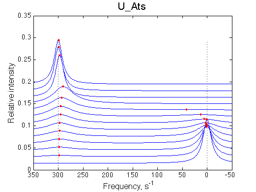 |
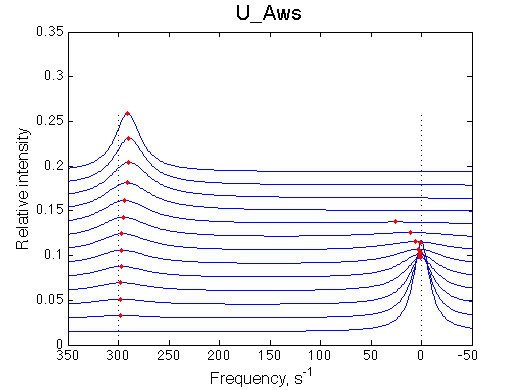 |
Looking at the late points in titration on the two lower graphs we notice that the peaks shift differently as well as display dramatic change in the line shapes for the weak and tight binding events. Most of the difference between two models appear at L/R range of about 0.7 to 1.1. I am showing the same graphs below again alongside with the corresponding population and line width plots:
 |
 |
 |
 |
 |
 |
Now we can re-design the titration series to emphasize the difference between the two models. We will not make any changes to the models and will add titration points near equimolar ratio of R and L. I will duplicate my setup.txt and rename that to setup2.txt. Here I will change L/R ratios used in the titration (LRratio) and change output folder (Results_Path). Now I re-run simulations by issuing
Simulate setup2 U_Aws, and
Simulate setup2 U_Ats
New simulation result is summarized in Example_simulation_2/summary_report.htm and I also show the graphs side-by-side below.
 |
 |
 |
 |
 |
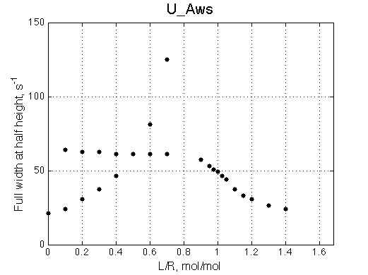 |
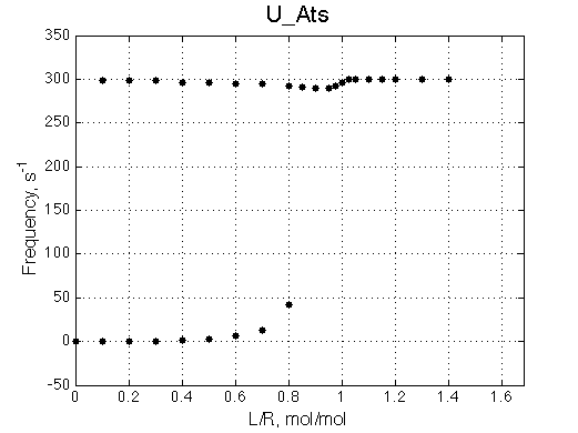
The two models produce substantially different line shapes at the chemical shift of RL complex emphasized by the additional titration points. The line width of the bound peak in tight-binding case U_Ats rapidly narrows from L/R=0.8 to 1 and quickly plateaus. In the weak binding case the peak is narrowing almost linearly from 0.8 to 1.2 even if at L/R=1.2 the formation of RL is 95% complete.
It is clear that the line width is extremely sensitive to the parameters of the binding event. Curiously, the line width curve of the bound from closely resembles an ITC profile calculated for these systems. However, this is only an apparent similarity highlighting the rapid changes near equimolar binding conditions. In fact, ITC profiles for 1:1 systems, however steep or shallow, always have a midpoint of the profile at L/R=1. In the tight binding case most of the changes occur before L/R=1 while in the weak binding - the L/R=1 occurs at some 1/4 of the total FWHH change.
 |
 |
Another curious observations is the shift of the RL resonance towards R, followed by a return to the true RL position as titration progresses.
 |
 |
 |
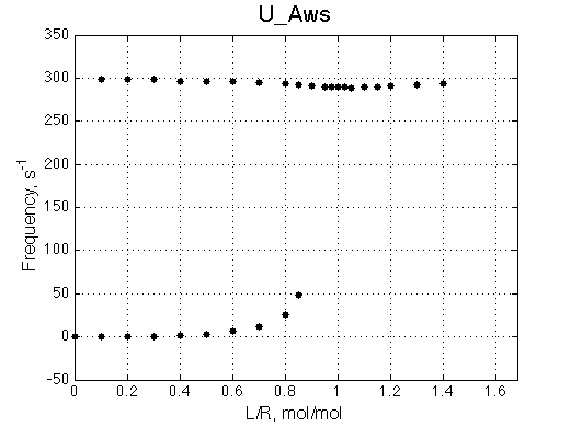 |
The reason for this late-in-titration shift of RL peak is quite simple. Generally, the exchange regime is defined by the relationship of the chemical shift separation between the exchanging species and the exchange rate constant, kex , which is a sum of the first-order forward and reverse rate constants: kex =kf +kr (Cavanaugh et al. 2006). Reverse rate constant k2 is a true first-order constant (so kr =k2) but forward one has to be computed as the pseudo-first order constant: kf =k1 *[L], thus including equilibrium concentration of L. In the beginning of titration [L] is very small so kex is dominated by kr which in this case is 20 s-1 < 300 s-1 , the chemical shift separation between R and RL, giving rise to the slow exchange regime with the two separate peaks for R and RL. However, at the end of titration [L] rapidly increases so value of kex is now dominated by kf shifting the exchange regime to intermediate, and eventually, to fast exchange. In the fast exchange two peaks coalesce into one at averaged frequency, weighted by populations of species at that titration point. Late in titration, when exchange shifts to the fast regime we have most of R in the RL form so the fast exchange average peak resides near RL position, slightly shifted towards R due to residual population of R. Visually it appears that as titration progresses the RL peak first occupies its true position, then shifts towards R and then comes back as all R is saturated with RL. In our example, saturation is achieved for U_Ats and not quite in U_Awf. Titration series needs to be extended to higher L/R to reach saturation in the weak binding case.
The immediate conclusion from this analysis is that the NMR-derived parameters of the two U systems is quite different even in slow exchange, normally thought of as the least sensitive range of conditions for NMR spectroscopy.
An appropriate design of a titration series, emphasizing late part of the titration, enables sensitive measurement of binding event characteristics.
Another useful outcome of the analysis of this simplest model is demonstration that routine analysis of NMR titration data done by just looking at chemical shift changes during titrations is highly unreliable and must be replaced with analysis of full NMR line shapes to extract correct information.
It is well known that chemical shift titration curves are only adequately representing accumulation of RL complex and may be fit to obtain equilibrium constant in the fast exchange regime. However, in practice it is quite difficult to guess where it is still adequate treatment and when it cannot be used. To illustrate the point I will simulate a few examples of the titration series when the off-rate gradually decreases.
Simulation report : summary_report.htm
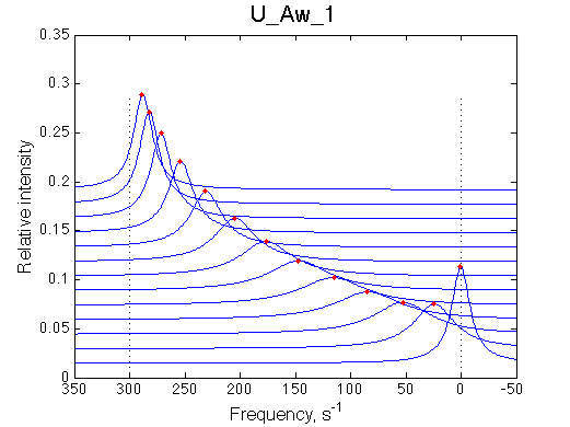
The first simulation represents a true fast exchange regime with k2 =500 > dw=300 s-1 . The spectral series shows a 'marching' peak from a position of R to RL as titration progresses. The chemical shift titration curve closely resembles curve of RL population as shown on the population graph just below. In this case, fitting of chemical shift curve will produce accurate equilibrium constant of RL formation.
| k2 , s-1 | NMR line shapes |
Chemical shift titration curve |
500 |
 |
 |
 |
As the exchange slows down and actually enters intermediate regime (k2 =300 = dw=300 s-1 ) one still can observe shifting average peak with much smaller intensity but yet detectable to build a chemical shift titration curve. The curve begins to show a 'lag phase' in the beginning of titration, which may mislead a researcher into thinking of a more complex binding mechanism (which could be 2-site binding, B model in LineShapeKin Simulation). Note that the difference in intensity loss of the peaks along the titration series is not dramatically different from the previous case.
| k2 , s-1 | NMR line shapes |
Chemical shift titration curve |
Line Width |
300 |
 |
 |
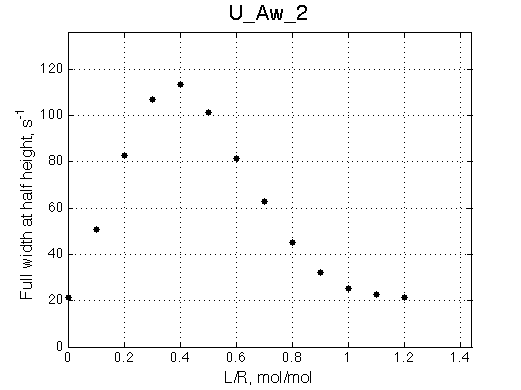 |
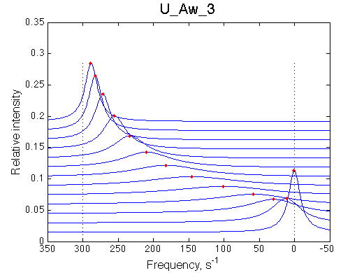
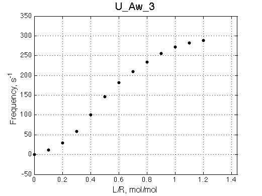
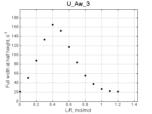
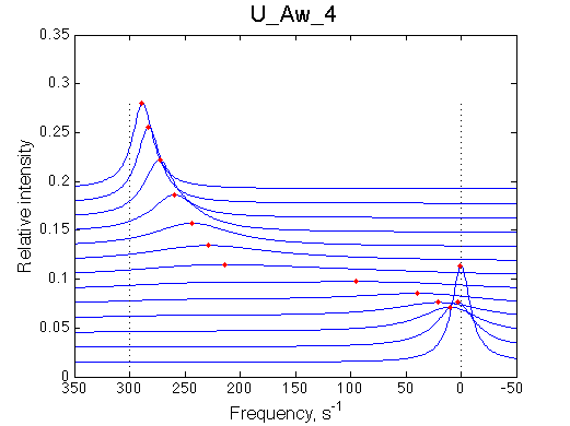
Here off-rate constant just dropped below chemical shift separation between R and RL (k2 =200 < dw=300 s-1 ). The peaks in the middle of titration are not going to be very visible in real spectra but what is detectable will certainly look like a sigmoidal profile, strongly suggesting 2-site binding mechanism.
| k2 , s-1 | NMR line shapes |
Chemical shift titration curve |
|
200 |
 |
 |
 |
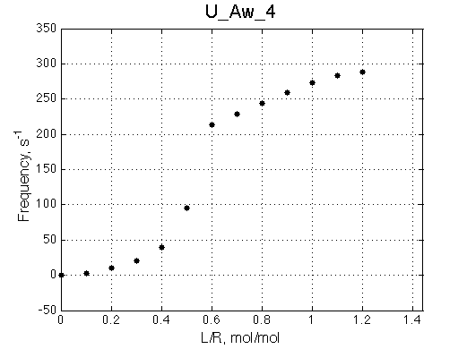
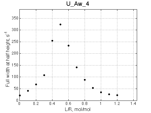
Off-rate constant of 100 s-1 finally renders chemical shift titration curve safely unusable for fitting of titration progress any more.
| k2 , s-1 | NMR line shapes |
Chemical shift titration curve |
|
100 |
 |
 |
 |
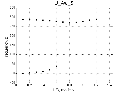
Below a final slow-intermediate exchange pattern is shown.
| k2 , s-1 | NMR line shapes |
Chemical shift titration curve |
50 |
 |
 |
The grand conclusion from this simple analysis is that it is extremely easy to be misled by appearance of the chemical shift titration curves for systems in near intermediate exchange regime. The only practical solution is to stop using chemical shift titration curves and use full line shape instead for analysis of the binding reaction mechanisms. To enable such analysis the LineShapeKin Analysis module has been developed that accepts HSQC data and fits them with variety of the models.
Having stated inadequacy of chemical shift titration plots, I will still make use of them in LineShapeKin Simulation for the purpose of illustrating the chemical shift evolution during titration progress in different model systems.
The simulated data are automatically exported in the format readable by LineShapeKin 3.2. This LineShapeKin version accepts 1D slices of a titration series and at the time of this writing only performs 2-site binding analysis. However, even if multi-site mechanisms are not implemented yet for the fitting it is instructive to explore how the data simulated for different mechanisms will be fit by a generic two-site model. This kind of analysis may be useful to learn how to recognize complex behaviors in HSQC spectra.
Here I will demonstrate how to fit the simulated data assuming the reader is a current user of LineShapeKin 3.2, which is available from http://lineshapekin.net/.
To separate this exercise from previous data we will use new U_A_lineshapekin.txt and setup_lineshapekin.txt. I will extend titration range LRratio to 2.0 to make sure the titration is complete (incomplete titrations may also be fit but see http://lineshapekin.net/ for this topic, specifically Examples of line shape fitting with different models: Determination chemical shifts of titration end point)
Issue Simulate setup_lineshapekin U_A_lineshapekin
Folder Example_fitting_test/ contains summary_report folder and a data folder U_A_lineshapekin/
The spectral simulations are filtered to remove excessive number of points along the baseline and save in LineShapeKin_3/ subfolder.
Copy from desired fitting model of LineShapeKin 3.2 into this folder:
Adjust model_setup.m
Adjust setup.m
Issue main
The fitting results are summarized in results/
Let's compare fitting results with the original simulation parameters:
Original simulation |
Fitting result with LineShapeKin 3.2 |
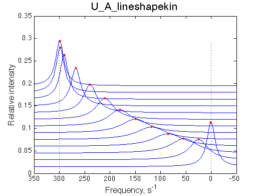 |
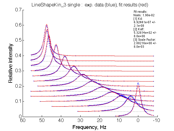 |
|
# Association constants # Rate constants of REVERSE reactions |
Optimum norm: 1.90e-02 Notice: 1. LineShapeKin reports Kd rather than Ka 2. units of frequency are Hz here. 4. the spectral slices have points filtered to remove exessive number of points at the baseline. |
We obtained Ka =1/Kd= 1.40-1.49 *106 M-1 and k2 =Koff=532+-8 s-1
This is a good result also telling us that the 95% confidence intervals on parameters determined by LineShapeKin are overly optimistic (need to be increased by factor of about 10 to encompass the true value of the simulation parameter, at least in this case).
Now let's compare chemical shift changes and line widths for the simulation and the fitted result (as another gauge of accuracy of the model)
Run new simulation to produce data using fitted parameters:
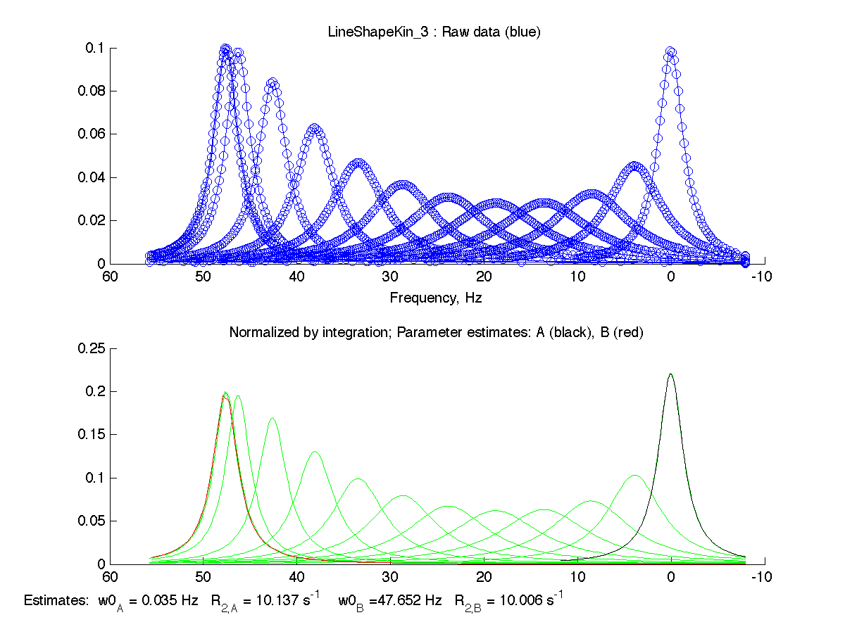
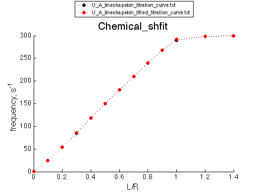
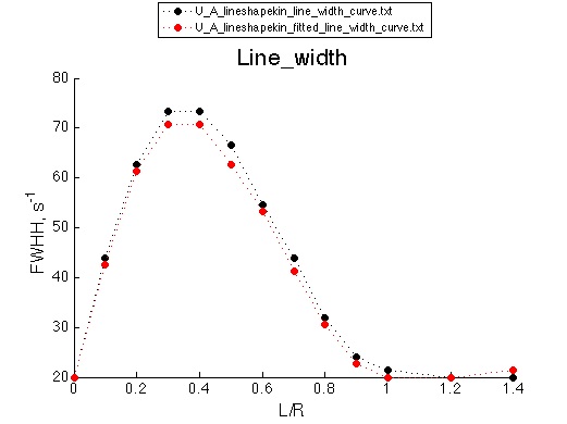
These graphs serve as additional goodness-of-fit indication, which will be utilized in the analysis of fitting of complex models with alternative binding mechanisms.
Back to LineShapeKin Simulation Tutorial