LineShapeKin

NMR Lineshape Analysis for Determination of Association Kinetics

General background and workflow outline

For overall outline of the program structure and its features see: my poster presentation on LineShapeKin at ICMRBS 2008 in San Diego, CA . The poster describes major features and uses in Version 3.1. For description of full capabilities, please, keep reading this online manual.  

Introduction

   Intermolecular interactions are characterized by equilibrium dissociation constant, K_d and kinetic constants of association and dissociation k_on and k_off. Binding event leads to changes in chemical shifts and line shapes of nuclei. Quantitative analysis of these changes allows one to describe kinetics of binding interactions.  HSQC or HMQC 2D-NMR experiments allow to simultaneously extract information from multiple independent probes in the protein (ie amide nitrogens, methyl carbons etc). Frequently a group of nuclei will respond to the same binding process and that allows to over-detemine the fitting problem and get most accurate results. In cases when there are multiple different binding interactions  occuring on protein surface, this technique gives site-resolved kinetic information which is inaccessible by most other means.

    LineShapeKin is set of Python and Matlab programs for analysis of NMR line shape in terms k_on and k_off.  It is advisable to determine macroscopic K_d by a separate technique such as Isothermal Titration Calorimetry (ITC) so to reduce number of fitting parameters and increase accuracy of the result. As an approximation, K_d may be determined by fitting of the peak positions to generate a titration curve (this only  works for peaks in fast exchange limit). Optionally, K_d may be fit together with k_off .

   LineShapeKin uses 1D line shape slices for fitting instead of full 2D line shape from HSQC 2D plane. The advantages of this approach is as follows:

• 'Slicing' of 2D lineshape in different dimensions w₁ and w₂ helps to resolve some overlaps.

  ---

• Amount of data is reduced quadratically so to facilitate simultaneous  fitting of  large number of residues.

  ---

• Obtaining 2 orthogonal 1D slices from the same peak over-determines the fitting problem (provided that both correlated nuclei experience the same binding event which is very likely so) .

    We use Sparky to handle spectral data and conveniently export 1D slices for desired set of peaks. NMRView has line-shape extraction module under development so check with Bruce Johnson (http://www.onemoonscientific.com/nmrview/). Future releases will include compatibility with other popular spectral analysis packages. Alternatively, the output of Sparky line-shape extraction module is plain text format files that may be produced by a user from any spectral-processing software.

Matlab notebooks perform raw data display, line-shape normalization, fitting to individual rate constants, fitting to global model with single set of K_d , k_on and k_off.  as well as statistical analysis.

Additionally to fitting different models LineShapeKin performs analysis of uniqueness of the 'best-fit' results. Direct Parameter Mapping  [3], the procedure originally introduced for analysis of relaxation dispersion data, is implemented in LineShapeKin to reveal mutual interdependce of the fitting parameters caused by the spefic exhange regime on the basis of the particular experimental spectral data set.

The typical workflow is:

• Export line-shapes of peaks that experience significant chemical shift changes using Sparky LineShapeKin extension.

  ---

• Normalize and scale spectral data in MATLAB. Obtain estimates of initial R₂ and w₀. Remove the 1D slices that have line shape distortions.

  ---

• Fit all the data individually in Matlab to see the distribution of the rate constants.

  ---

• Remove peaks that could not be fit well because of shape/overlap problems.

  ---

• Fit globally the groups that displays similar kinetics.

  ---

• Perform statistical analysis (using Akaike's Information Criterion) to determine whether data support better a single global or multiple individual sets of kinetic constants.
  

More detailed workflow is as follows

• Spectral data is displayed in Sparky and the custom extension is used to 'slice' peaks. You enter consequtive numbers in the list of spectra to let LineShapeKin know the sequence of experiments. To determine the line shape region to use you draw a rectangle around the peak and then integrate one of the dimensions. All individual spectra will manually or automatically produce a set of 1D traces that will be handled by Matlab as a single dataset.

  ---

• The integrated data are saved to disk in the folder Data_for_Matlab/:
  
• folders for every peak/dimension XNNN_x_w?/
  (where XNNN is residue name, x_w? stands for what dimension is x-axis in this 1D-trace, i.e. N97_x_w1 for 1D along w1)
• plain text files numbered with consecutive numbers of titration points (user supplied)
• points_list.txt - a list of names (numbers) of experiments in the series. It will be read by Matlab to load data files (above). User may remove any points from this list and the corresponding data files will NOT be used in subsequent fitting. This is to deal with problems of partial overlap during titrations.
  
• matlab.peaklist file containing a string of saved peak slices formatted so to directly cut-and-paste to setup.m
• If you keep Data_for_Matlab/ with your Sparky project you will be able to quickly go back and forth between Sparky and MATLAB to optimize specific spectral slice. However, sometimes it is convenient to move this folder after line shape extraction is finishd to a different location to prevent accidental changes. You will set path to it in setup.m

  ---

  
  
• Matlab directories and files:
• code/ and DPM_code/ - LineShapeKin libraries. You should set path to them in Matlab:File:Set Path.
• Setup.m is a control file for the package. Modify Sparky_path value in setup.m to point at the directory with your Sparky project.
• Models are set by using specific files:
  • model_setup.m - file with model parameters.
  • rate_matrix.m - file with the function that builds all model -relevant matrices

• More technical information about Matlab files is given in Technical_Description

Back to the top

References and how to cite

So far I did not write a paper specifically describing the package. However, please, cite reference [1] where the major functionality of the LineShapeKin was used.  The early version of LineShapeKin was based on the code developed by Roger Cole and Patrick Loria [2]. I also greatly acknowledge Dr. James G. Kempf for helpful discussions. Direct Parameter Mapping technique was introduced and described in [3].

The internal formalism of LineShapeKin is based on classic treatment of chemical exchange. For review and detailed discussion see [4,5] though this list is by no means exhaustive. 

1. Kovrigin, E.L. and Loria, J.P., Enzyme dynamics along the reaction coordinate: Critical role of a conserved residue. Biochemistry, 2006. 45(8): p. 2636-2647.
2. Beach, H., Cole, R., Gill, M.L., and Loria, J.P., Conservation of mu s-ms enzyme motions in the apo- and substrate-mimicked state. Journal of the American Chemical Society, 2005. 127(25): p. 9167-9176.
3. Kovrigin, E.L., Kempf, J.G., Grey, M.J., and Loria, J.P., Faithful estimation of dynamics parameters from CPMG relaxation dispersion measurements. Journal of Magnetic Resonance, 2006. 180(1): p. 93-104.
4. Cavanaugh, J., Fairbrother, W.J., Palmer III, A.G., and Skelton, N.J., Protein NMR Spectroscopy: Principles and Practice. 2006: Academic Press. 587.
5. Fielding, L., NMR methods for the determination of protein-ligand dissociation constants. Progress in Nuclear Magnetic Resonance Spectroscopy, 2007. 51(4): p. 219-242.

Back to the top

Protocol of line shape analysis

• Preparation of the experimental HSQC titration data
• LineShapeKin Sparky extension for extraction of spectral data
• Data analysis in MATLAB (individual fitting)
• Global (group) data fitting

Preparation of the experimental HSQC titration data

1. Process the data with sufficient zero-filling to obtain 15-20 data points per peak envelope.
   
   
   1. IMPORTANT NOTE 1: Additional points will decrease speed of calculations and may  cause 'Out of Memory Error' in Matlab when analyzing multiple residues. You should zero-fill, if you have low resolution, to 10-20 points per peak envelope to enhance robustness of the fitting procedure. Further zero-filling will only decrease performance.

      ---

   2. IMPORTANT NOTE 2: The same effect may be seen if you include too much of a baseline. You should use relatively small region just around the peak to keep data size minimal as describe in LineShapeKin Sparky extension for extraction of spectral data.
      

   ---

2. Use EM apodization window (exponential multiplication) to keep line shapes in the frequency dimension lorentzian. Any other window-functions will result in poor fits. Avoid using proton dimension if there is proton-proton splitting evident in the peak line shape.
   

   ---

3. Use a batch processing nmrPipe script to have identically processed series of HSQC spectra.

   ---

Back to Protocol section

Back to the top

LineShapeKin Sparky extension for extraction of spectral data

(separate document)

Data analysis in MATLAB (individual fitting)

Introduction

This manual has been written along with the development of the package so some text became obsolete but has been overlooked and not deleted. If you find difficulty reproducing some step, please, read on as the same topic is often discussed more than once and that will take you to more updated info. If still something is not working as described, please, let me know (write to )

1. Make a new directory where your line shape analysis results will be saved.

   ---

2. Go into LineShapeKin/Docs/Setup_Examples. This folder contains examples of data fitting with different models. Next
   1. choose the model you want to work with (I recommend to begin here with 1.Matlab_fitting.Koff_SF, which is two-site exchange, K_d is preset while K_off and Scaling Factor are variable parameters), and
   2. copy all m-files you see there into your working directory.
      (For description of m-files see Technical_Description)

      ---

3. Start matlab and set File:Set Path to your working directory.
   You may want to try alternative ways of fitting the same spectral data. To do this just make separate working directories (with m-files corresponding to different models) and set them as working folders in different fitting sessions.

   ---

4. Set paths in Matlab (File:Set Path) to the lineshape analysis package code folder code/.
   

   ---

5. Open setup.m in Matlab :
1. Insert path to your slices created in the Sparky project into Sparky_data_path.
2. Cut-and-paste the string of slice-names from /Data_for_matlab/matlab.peaklist to setup.m resnames array.
   (this is where Matlab gets to know about the datasets you saved from Sparky. You don't need to put here entire list. You may put just one or two dataset names for the start - it is totally flexible. Additionally, after you have a few dataset names in there you still are able to display or fit just one of them - see below. You may come back to sparky and re-do integration for the dataset that is already entered in this list - Matlab will use newly exported data).
   

   ---

   
   
   
   
6. Check quality of the Sparky-exported dataset before attempting to fit the data:

   ---

1. Set project_name= 'just display data' mode (uncomment the string and make sure other choices below are commented out )  and set residue_number to serial number of residue name in resnames .

   ---

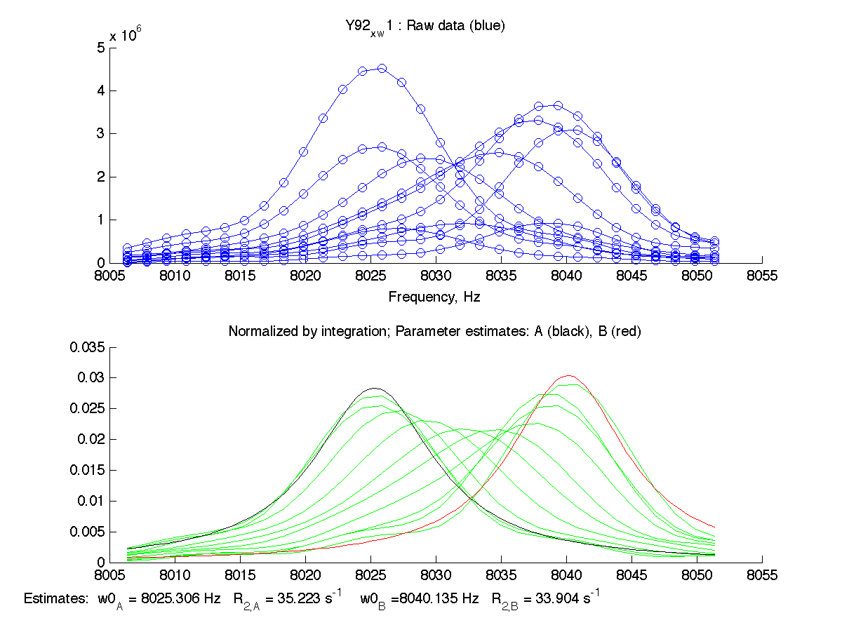
2. issue main on a MatLab command line. The program plots the raw spectral data and tries to estimate frequencies and line widths (as apparent relaxation rates) for starting and ending state. Resulting estimates are shown on the bottom of the graph with black trace for initial (A) state and red trace for final (B) state:
   

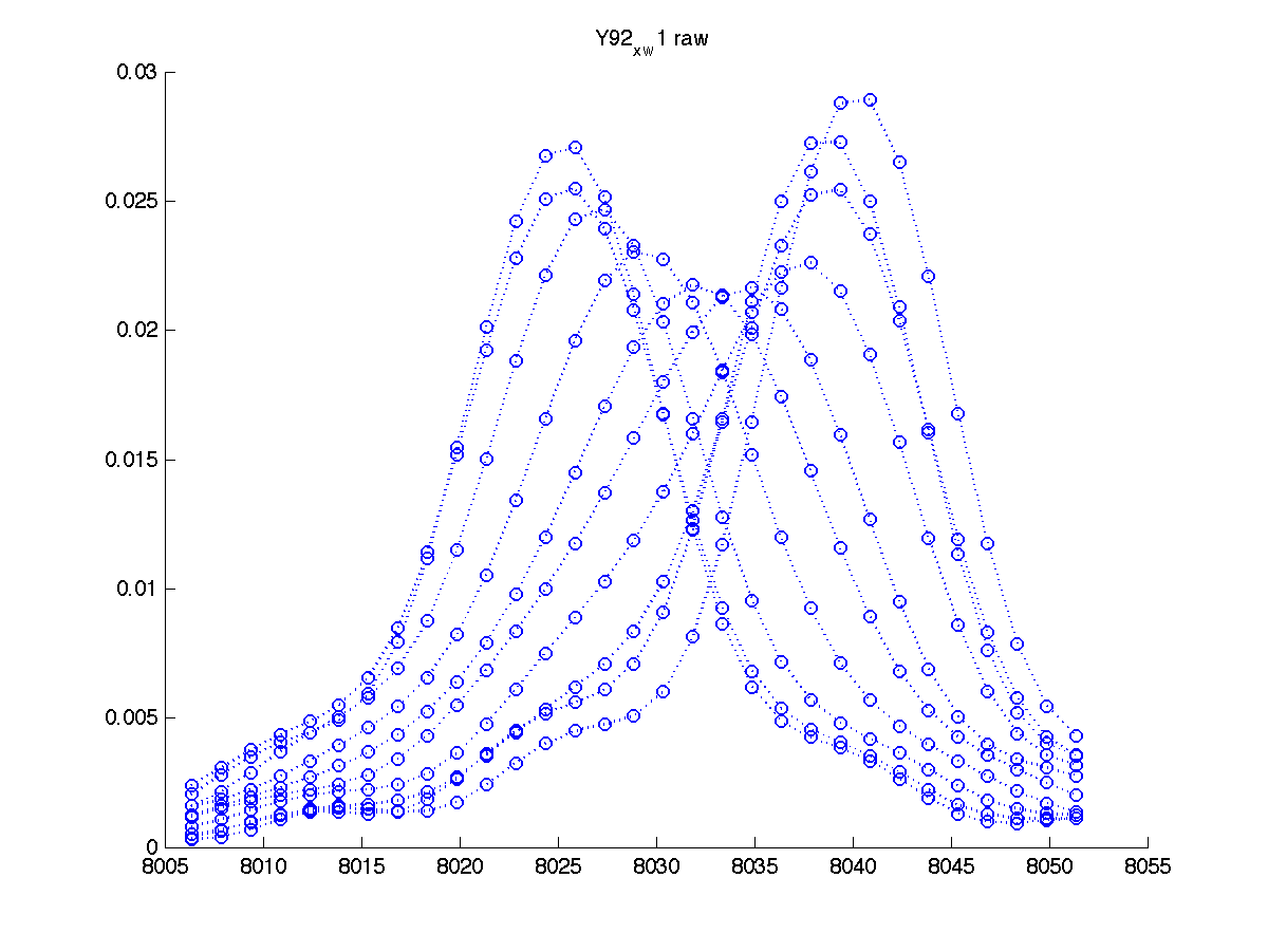
   You also get another graph to more closely inspect individual traces:

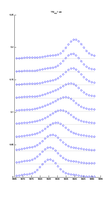
   If  you use plotting option (setup.m) Stacked_Plot=YES you can display the titration series stacked rather than overlayed with another option setting shift of traces in units of relative peak height Percent_Shift=75. For this graph to be more useful - you should stretch the window of the MATLAB figure vertically like this: If you want to export it, make sure you adjust Width/Height options in the Export menu of Matlab.

   
   The program displays raw data set and attempts to normalize it . NOTE: Both 1D slices are reversed due to opposite direction of X-axis in NMR and in regular Cartesian coordinate system.
   

First step before fitting is to normalize peak areas within a titration series for one residue. The issue is that we integrate some number of raw spectral points (defined by a specific rectangle width) that lead to artificial different intensities in a series. However, we exploit the basic fact that the peak area is independent of its shape and constant for the series of 1D slices for one residue. Therefore LineShapeKin estimates peak areas within the titration series via rectangular or Simpson's integration formula and normalizes areas of all 1D slices to unity. This approach also allows to remove effect of exchange broadening in the other dimension. If we are looking at proton dimension trace, the effect of exchange broadening in nitrogen dimension is that peak intensity drops more significantly in proton slice as well reducing the integrated area. We should either explicitly take it into account or remove it by exploiting the property of NMR signal that its area is proportional to the number of nuclei in the sample no matter what line shape is. The LineShapeKin takes the latter approach.

---

3. You may drop any titration point from fitting if the line shapes are distorted by (transient) overlap in some spectra. Simply remove titration point indices from XNNN_x_w?/points_list.txt. You may include them back for fitting at any time because the spectral data are not removed.

   ---

4. The program also estimates chemical shifts of initial (A) and final (B) states (w0_A and w0_B) as well as corresponding R2s of pure states using first and last peaks in the series by fitting them to lorentzians. These estimates are used as constants later in actual line shape fitting to McConnel equations. Therefore it is critical to obtain good estimates at this step.

   ---

5. If the estimates of A and B peak positions and line widths look really bad you should return back to Sparky and slice peak again taking this time some more (or less) baseline around the peak (using longer or shorter rectangle). Most of the time it is possible to achieve good initial estimates by changing the way you slice the peak. However, it is the least formalized part - you should try different possibilities to achieve better results. Remember, the peak positions and relaxation rates for A and B states estimated at this step will be set  to fixed values in the next fitting runs and no longer adjusted (unless your model fits frequency of B state, w0_B parameter). Therefore it is important to achieve good estimates at this step.
   
   

   ---

6. Now just reissue main (no adjustment to setup.m is needed) and see if new set of 1D slices is fit better, thus providing adequate R2_A, R2_B and w0_A, w0_B estimates.

   ---

7. If the end points of titration series contain more than one peak (slow exchange regime when you see both A and B species) then automatic estimates for peak positions and R2 will fail. Same if your titration did not reach saturation but you can reasonable estimate w0_B from a titration curve. In these cases you have to turn off automatic estimation of chemical shifts and/or R2s of two end states A and B separately for each residue:
   1. insert known chemical shifts (in Hz) into XNNN_x_w?/manual_w0.txt file. Matlab will use these numbers and will skip automatic estimation by fitting.

      ---

   2. You may estimate R2 of A and B states as 3.1415*FWHH (full width at half height)and insert them into XNNN_x_w?/manual_R2.txt file in units rad/s . NOTE: These R2 are usually larger than real R2 you can measure in relaxation experiments due to finite acquisition time and use of apodization window. Matlab will use these numbers and will skip automatic estimation by fitting to lorentzians.

      ---

   3. If either of R2 or w2 files left empty LineShapeKin will try to fit the data and then will reset fitted parameters with the ones found in non-empty manual_??.txt file.  Matlab will plot the peaks corresponding to these numbers as black (A) and red (B) trace so you can check sanity of your estimates. If fitting fails you should supply estimates for both parameters.

      ---

   4. If peaks fit OK but you know that titration is not finished then  let it fit the initial and the end state frequencies and R2s. Later you will direct Matlab to fit the actual frequency of the end state while still using estimated R2 (see examples).

      ---

   5. If estimates are still unsatisfactory: enter both R2 and w2 values. This completely overrides automatic estimates and you may continue with fitting for k_off, which will start with your numbers instead.

      ---

   6. You may also switch project to Simulation Mode and observe what kind of line shapes you may expect for this residue and given Kd and koff.

      ---

   7. Troubleshooting:
      

      If the spectra do not fit well try :

      1. vary LINE_WIDTH_0. Set it to 20, 40 , 60 , 100 etc. and see the result with each value. There may be a problem if line witdths in two dimensions are significantly different an then with each setting of LINE_WIDTH_0 one dimension fits fine for different peaks and the other one consistently fails.  Try to find intermediate value. So far dataset-specific starting line widths for global datasets are not implemented.

      2. Try to 'slice' differently. Success of fitting may be extremely sensitive to the specific way you integrate a 1D slice. Try grabbing more or less of a baseline. Fast exchangers may need more baseline included. However, sometimes cutting peak just around it works better. Another version of 'slicing' is to include baseline only on one side of a peak and cut right after the peak on the other side (this way you increase percentage of points actually describing peak envelope).

      
      
      
      
      
      
7. Fitting a set of 1D slices:
   

   ---

   1. Use the model with
   • fixed K_d (if you know it from ITC) and variable k_off and Scale Factor from 1.Matlab_fitting.Koff_SF/ (see example), or

     ---

   • variable K_d , k_off and Scale Factor from 2.Matlab_fitting.Koff_Kd_SF/ (see examples)

     ---

1. Set the starting parameters of the model (K_d , k_off etc) in model_setup. Define (or accept default) which parameter is subject to a grid search and insert proper range for a grid search. The program will start fitting from every grid point independently to look, which optimization gave the best (smallest) norm and will do final optimization run starting from the lowest-norm results. Note, that procedure of grid search is quite time consuming (fit time x number of grid points). I DON'T RECOMMEND turning this feature off as it ensures that you will find a GLOBAL minimum rather than get stuck in a local one. However, if fitting takes too long - you may reduce number of grid points to just one to get quicker preliminary results and then rerun the fitting last time with the proper grid set.

   ---

2. Set project_name= 'single' mode  and residue_number=N,  NORMALIZATION='trace integration',
   BASELINE_CORRECTION=NO.
   




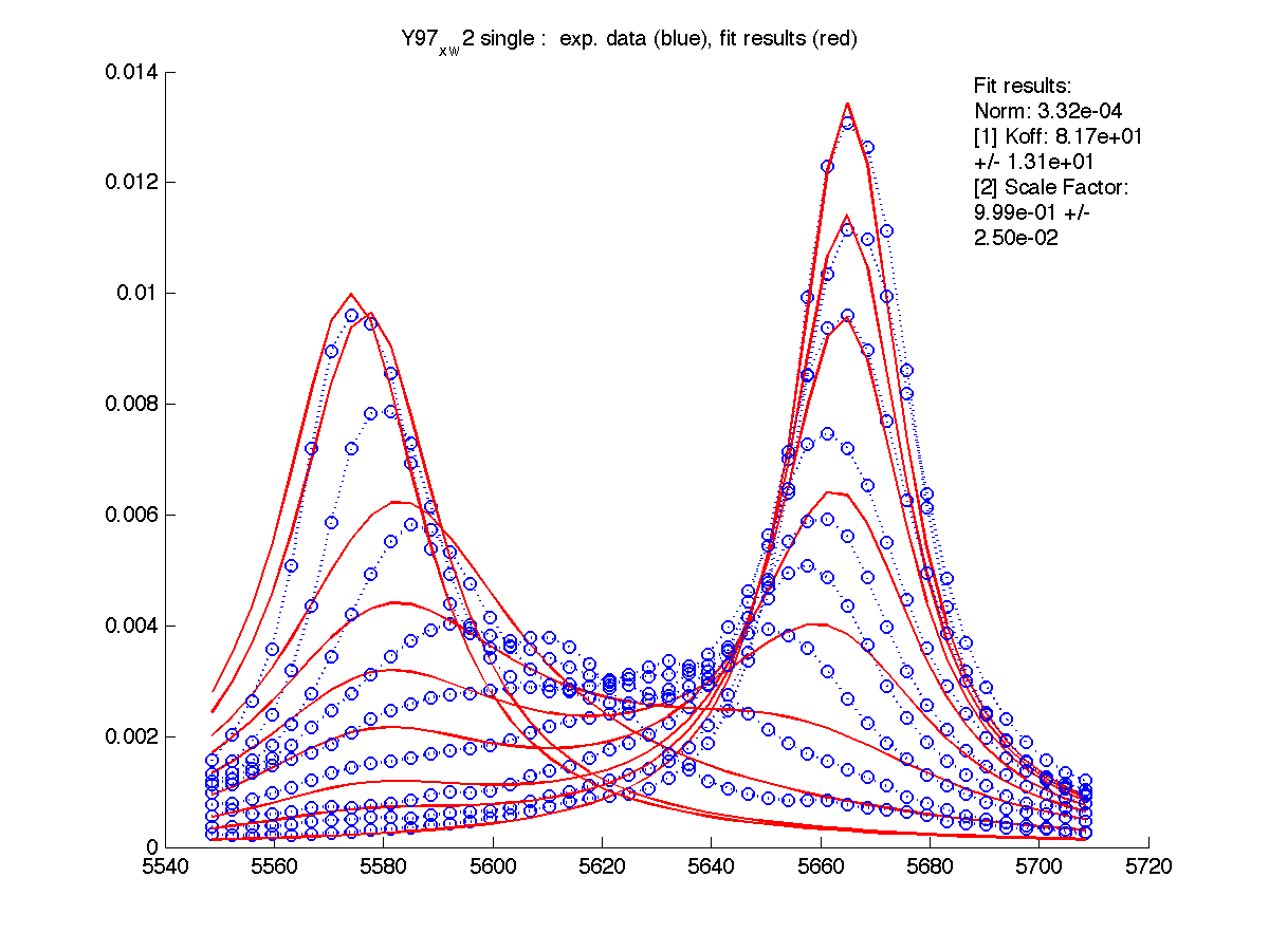
1. The program shows two graphs - raw data (you saw it previously) and fitting results. It saves them in figures/ as both PNG image and FIG file editable in Matlab.
   
   

   ---

2. Fit results are saved in a text format  in grid_results....dat files so you can check if the minimum you found is indeed global in a parameter space.
   

   ---

3. After you are satisfied with the fitting result for this residue you should enter the determined Scale Factor into XNNN_x_w?/scale_factor.txt file. This is a factor to compensate for our practical inablility to include entire lorentzian envelope in peak integration. The smaller fraction of the peak envelope is included - the larger this Scale Factor will be. If you put it into the above file, then raw data for this set of 1D slices will be scaled upon reading from disk and no scaling will be needed  any more. This will not change fitting parameters but will bring fitted value of Scale Factor to 1 (because data is already corrected).
   Please, note that this factor is specific for the particular slice you took in Sparky. If you re-do 'slicing' this scaling factor will be reset to 1 an you will have to determine it again.

   Here I entered Scale Factor of 2.23 into Y97_x_w2/scale_factor.txt. and rerun fitting. Now Scale Factor comes up as 0.99 and may be dropped from the model as a fitting parameter.

4. Setting proper Scale Factor for every dataset means that all residues will have identical peak areas which enables good fitting performance when you analyze global hypothesis (a few residues to be fit to the same K_d and k_off combination).

   ---

5. Now you can re-run calculations with reduced number of parameters (minus Scale Factor) and obtain K_d and K_off with better accuracy using model from  3.Matlab_fitting.plus_Kd.minus_SF/.




---

 

Back to the Protocol section

Back to the top

 

 

 

 

 

---

Global (group) data fitting

1. When finished individually fitting all the peaks and having set Scale Factor to the fitted values for every dataset you are ready to test hypothesis of global binding event versus hypothesis of localized independent binding events. We will fit data to individual k_off values for every residue and the fit them all together to a single koff , K_d combination . In order to do this: 
2. Set project_name='indiv' - to re-run fitting ofall of them individually to individual k_off-s with the adjusted scaling factor.   This fitting mode will reuse all manual adjustments to w0 and R2 as well (if you made them).

   ---

   1. set project_name='global' - to use one k_off. and fit them again. To do statistical testing - proceed to the next chapter.

      ---

 

Hints :

---

1. The group you fit globally may be independent residues as well as 2 dimensions of the same peak.

   ---

2. Try to integrate as narrow dimension as possible through the peak maximum - this way you retain best S/N.

   ---

3. Try both dimensions separately for the same residue: sometimes one works better than the other.

   ---

Back to the Protocol section

Back to the top

Statistical comparison of individual and global fitting results
(separate document)

Back to the Protocol section

Back to the top

Fitting of K_d , k_off  and the frequency of the B (bound) state resonance

 

1. You may also fit the position of the B state as your titration may be unfinished. Use model from 4.Matlab_fitting.plus_Kd_v0.minus_SF/ and see example
2. Make sure you test this fitting result versus 2-parameter model (Kd and Koff only) see here to determine whether additional fitting parameter is warranted by improvement of the fit.

   ---

3. NOTE: in this mode you cannot use global fitting mode (project_name= 'global') as every residue should  have its own specific frequency for the B state. However, it is possible to plug the fitted w0_B values into the 'manual_w0.txt' files (that are individual for every residue) and switch back to two-parameter (Kd,Koff) fitting model which now will use fixed resonance frequencies from these files, rather than from estimates. Use the model from 5.Matlab_fitting.plus_Kd.fixed_v0.minus_SF/ and see examples.
4. Now you can do testing of individual vs. global fitting hypothesis (see example).

Back to the top

Fitting of four parameters: Kd, Koff, frequency and correction to L/P ratio

1. The model definition may be extended to fit additional parameters such as correction to L/P ratio. It may come useful if concentrations of the binding partners are not precisely known.
2. Use model files from 7.Fitting.Kd.Koff.w0B.LPcorr and then test likelihood that this model is better than simpler one see here

Back to the top

Difficult cases

Overlaps:

Main problem is how to normalize peak areas for fitting:

• In general, if the overlap occurs in the spectrum you still can try to slice you peak in one of the dimensions on a shoulder such that overlap does not particularly contribute to the slice. When you slice a shoulder you will have lower signal/noise but cleaner line shape.
• The integration procedure seems to be efficient and stable even if you only slice the very top of the peaks. However, you may need fixing the frequencies and/or linewidths  (in manual_R2.txt and manual_w0.txt ) to enable quality fitting result.
• See an example here

  ---

Last updated on 3/28/08